The package Biogeme (biogeme.epfl.ch) is designed to estimate the parameters of various models using maximum likelihood estimation. It is particularly designed for discrete choice models. In this document, we present step by step how to specify a simple model, estimate its parameters and interpret the output of the software package. We assume that the reader is already familiar with discrete choice models, and has successfully installed PythonBiogeme. This document has been written using PythonBiogeme 2.5, but should remain valid for future versions.

1 The data file

Biogeme assumes that the data file contains in its first line a list of labels corresponding to the available data, and that each subsequent line contains the exact same number of numerical data, each row corresponding to an observation. Delimiters can be tabs or spaces. The tool biopreparedata can be used to transform a file in Comma Separated Version (CSV) into the required format. The tool biocheckdata verifies if the data file complies with the required format.

The data file used for this example is swissmetro.dat. Note that the first time a data file is used by Biogeme, it is compressed and saved in binary format in a file. The name of this file is the same as the original file, preceeded by __bin_. In our example, the binary file is __bin_optima.dat. If the original text file is modifed, the binary file must be erased from the directory in order to account for the changes. The name of the file that has actually been used is reported in the output file.

Biogeme is available in two versions. BisonBiogeme is designed to estimate the parameters of a list of predetermined discrete choice models such as logit, binary probit, nested logit, cross-nested logit, multivariate extreme value models, discrete and continuous mixtures of multivariate extreme value models, models with nonlinear utility functions, models designed for panel data, and heteroscedastic models. It is based on a formal and simple language for model specification. PythonBiogeme is designed for general purpose parametric models. The specification of the model and of the likelihood function is based on an extension of the python programming language. A series of discrete choice models are precoded for an easy use.

In this document, we describe the model specification for PythonBiogeme.

2 The model

The model is a logit model with 3 alternatives: train, Swissmetro and car. The utility functions are defined as:

where TRAIN_TT_SCALED, TRAIN_COST_SCALED, SM_TT_SCALED, SM_COST_SCALED, CAR_TT_SCALED, CAR_CO_SCALED are variables, and ASC_TRAIN, ASC_SM, ASC_CAR, B_TIME, B_COST are parameters to be estimated. Note that it is not possible to identify all alternative specific constants ASC_TRAIN, ASC_SM, ASC_CAR from data. Consequently, ASC_SM is normalized to 0.

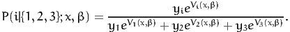
The availability of an alternative i is determined by the variable y_i, i=1,...3, which is equal to 1 if the alternative is available, 0 otherwise. The probability of choosing an available alternative i is given by the logit model:

(1)

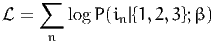
Given a data set of N observations, the log likelihood of the sample is

(2)

where i_n is the alternative actually chosen by individual n.

3 Model specification: PythonBiogeme

The model specification file must have an extension .py. The file 01logit.py is reported in Section A.1. We describe here its content.

THe objective is to provide to PythonBiogeme the formula of the log likelihood function to maximize, using a syntax based on the Python programming language, and extended for the specific needs of Biogeme. The file can contain comments, designed to document the specification. Comments are included using the characters #, consistently with the Python syntax. All characters after this command, up to the end of the current line, are ignored by PythonBiogeme. In our example, the file starts with comments describing the name of the file, its author and the date when it was created. A short description of its content is also provided.

These comments are completely ignored by PythonBiogeme. However, it is recommended to use many comments to describe the model specification, for future reference, or to help other persons to understand the specification.

The specification file must start by loading the Python libraries needed by PythonBiogeme. Two libraries are mandatory biogeme and headers. The first includes the extension of the PYthon programming language needed by PythonBiogeme. The second imports the names of the headers of the data file, so that they can be directly used in the specification of the model. In this example, an additional library is loaded as well: statistics. It implements some functions that report statistics about the data file.

The next statements use the function Beta to define the parameters to be estimated. For each parameter, the following information must be mentioned:

1. the name of the parameter,
2. the default value,
3. a lower bound,
4. an upper bound,
5. a flag that indicates if the parameter must be estimated (0) or if it keeps its default value (1),
6. a description of the parameter, to be used in the LATEX report.

Note that, in Python, case sensitivity is enforced, so that varname and Varname would represent two different variables. In our example, the default value of each parameter is 0. If a previous estimation had been performed before, we could have used the previous estimates as default value. Note that, for the parameters that are estimated by PythonBiogeme, the default value is used as the starting value for the optimization algorithm. For the parameters that are not estimated, the default value is used throughout the estimation process. In our example, the parameter ASC_SM is not estimated (as specified by the 1 in the fifth argument on the corresponding line), and its value is fixed to 0. A lower bound and an upper bound must be specified. By default, we suggest to use -1000 and 1000. If the estimated value of the parameter happens to equal to one of these bounds, it is a sign that the bounds are too tight and larger values should be provided. However, most of the time, if a coefficient reaches the value 1000 or -1000, it means that its variable is poorly scaled, and that its units should be changed.

Note that none of the Python variables is used by PythonBiogeme. They are used only to simplify the writing of the formula. Therefore, nothing prevents to write

and to use car_cte later in the specification. The variable car_cte will be unknown by PythonBiogeme and will not appear in any reporting file. We strongly advise against this practice, and suggest to use the exact same name for the Python variable on the left hand side, and for the PythonBiogeme variable, appearing as the first argument of the function, as illustrated in this example.

It is possible to define new variables in addition to the variables defined in the data files. It can be done either by defining Python variables using the Python syntax:

It can also be done by defining PythonBiogeme variables, using the function DefineVariable.

The latter definition is equivalent to add a column with the specified header to the data file. It means that the value of the new variables for each observation is calculated once before the estimation starts. On the contrary, with the method based on Python variable, the calculation will be applied again and again, each time it is needed by the algorithm. For small models, it may not make any difference, and the first method may be more readable. But for models requiring a significant amount of time to be estimated, the time savings may be substantial.

When boolean expressions are involved, the value TRUE is represented by 1, and the value FALSE is represented by 0. Therefore, a multiplication involving a boolean expression is equivalent to a “AND” operator. The above code is interpreted in the following way:

• CAR_AV_SP is equal to CAR_AV if SP is different from 0, and is equal to 0 otherwise. TRAIN_AV_SP is defined similarly.
• SM_COST is equal to SM_CO if GA is equal to 0, that is, if the traveler does not have a yearly pass (called “general abonment”). If the traveler possesses a yearly pass, then GA is different from 0, and the variable SM_COST is zero. The variable TRAIN_COST is defined in the same way.

Variables can be also be rescaled. For numerical reasons, it is good practice to scale the data so that the values of the estimated parameters are around 1.0. A previous estimation with the unscaled data has generated parameters around -0.01 for both cost and time. Therefore, time and cost are divided by 100.

We now write the specification of the utility functions.

We need to associate each utility function with the number of the alternative, using the numering convention in the data file. In this example, the convention is described in Table 1. To do this, we use a Python dictionary:

We use also a dictionary to describe the availability conditions of each alternative:

We now define the choice model. The function bioLogLogit provides the logarithm of the choice probability of the logit model. It takes three arguments:

1. the dictionary describing the utility functions,
2. the dictionary describing the availability conditions,
3. the alternative for which the probability must be calculated.

In this example, we obtain

We next defined an iterator on the data using the statement

and define the ESTIMATE variable of the BIOGEME_OBJECT with the formula of the log likelihood function:

Other variables can be defined in the BIOGEME_OBJECT. In particular, the EXCLUDE variable allows to ignore some observations in the data file. It contains a boolean expression that is evaluated for each observation in the data file. Each observation such that this expression is “true” is discarded from the sample. In our example, the modeler has developed the model only for work trips, so that every observation such that the trip purpose is not 1 or 3 is removed. Observations such that the dependent variable CHOICE is 0 are also removed. Remember the convention that “false” is represented by 0, and “true” by 1, so that the ‘*’ can be interpreted as a “and”, and the ‘+’ as a “or”. Note also that the result of the ‘+’ can be 2, so that we test is the result is equal to 0 or not. The exclude condition in our example is therefore interpreted as: either (PURPOSE different from 1 and PURPOSE different from 3), or CHOICE equal to 0.

Note that we have conveniently used an intermediary Python variable exclude in this example. It is not necessary. The above statement is completely equivalent to

The variable PARAMETERS allows to define various parameters controlling the configuration of PythonBiogeme. In this example, we have selected to use the optimization algorithm BIO using the following syntax.

The variable FORMULAS is used to select the parts of the model specification that are reported in the report file. In general, the formula of the log likelihood function is too complicated to be readable, and it is preferred to report only the specification of the utility functions, as in this example.

Finally, we request PythonBiogeme to calculate some statistics about the null log likelihood, the log likelihood of a model with constants only, and statistics about the availability of the alternatives.

The function nullLoglikelihood computes the null loglikelihood from the sample and ask PythonBiogeme to include it in the output file. The first argument is a dictionary mapping each alternative ID with its availability condition. The second is an iterator on the data file. The result is the log likelihood of a model where the choice probability for observation n is given by is 1∕J_n, where J_n is the number of available alternatives, i.e.

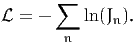(3)

The function cteLoglikelihood computes the constant loglikelihood from the sample and ask PythonBiogeme to include it in the output file. It assumes that the full choice set is available for each observation. The first argument is a list containing the alternatives in the choice set. The second argument is the choice expression producing the id of the chosen alternative. The third argument is an iterator on the data file. The result is the log likelihood of a logit model where the only parameters are the alternative specific constants. If n_i is the number of times alternative i is chosen, then it is given by

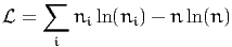(4)

where n = ∑ _in_i is the total number of observations.

The function availabilityStatistics computes the number of times each alternative is declared available in the data set and ask PythonBiogeme to include it in the output file. The first argument is a dictionary containing for each alternative the expression for its availability. The second is an iterator on the data file. The result is a dictionary D with an entry D[i] for each alternative i containing the number of times it is available.

4 Running PythonBiogeme

The estimation of the model is performed using the following command

The following information is displayed during the execution.

• Some information about the version of Biogeme.
  This is biogeme (pythonbiogeme) 2.5
• The name of the sample file that is read.
   Read sample file: swissmetro.dat
• PythonBiogeme is able to use several processors if they are available. By default, it uses half of the number fo available processors on the computer.
   Nbr of cores reported by the system: 4 
   Nbr of cores used by biogeme: 2
• The details about the iterations of the estimation procedure are reported.
   Init. log-likelihood: -6964.66 [00:00] 
       gmax Iter   radius        f(x)     Status       rhok nFree 
   +1.44e-01    1 1.00e+00 +6.9646630e+03 ****Converg  +1.07e+00 4  ++ P 
   +5.29e-02    2 2.00e+00 +5.4217993e+03 ****Converg  +1.08e+00 4  ++ P 
   +9.43e-03    3 4.00e+00 +5.3328087e+03 ****Converg  +1.02e+00 4  ++ P 
   +2.34e-04    4 8.00e+00 +5.3312529e+03 ****Converg  +1.00e+00 4  ++ P 
   
   Convergence reached... 
  --> time interval [16:28:46,16:28:46]
• The value of the parameters at the end of the iterarions.
   Estimated parameters: 
  ASC_CAR = -0.154633 
  B_TIME = -1.27786 
  B_COST = -1.08379 
  ASC_SM = 0 
  ASC_TRAIN = -0.701187

The following files are generated by PythonBiogeme:

• 01logit.html: the results of the estimation in Html format. Its content is described in Section 5.
• 01logit_param.py: the estimated value of the parameters, together with the variance-covariance matrix of the estimates, in a syntax that can be directly reused in a model specification file.
• 01logit.log: a file containing messages produced by PythonBiogeme during the run.
• 01logit.tex: a file containing the main results in LATEX format. See Table 2.
• hess.lis: contains the final BHHH and the second derivative, or Hessian, matrix. The format is such that it can be copied and pasted in a matrix language such as Matlab or Octave.
• hessian.lis: contains the (opposite of the) Hessian matrix of the log likelihood function at each iteration, in a Matlab compatible format.
• __parametersUsed.py: provides an exhaustive list of the parameters used by the run of PythonBiogeme, together with the value that has been used.

In order to avoid erasing previously generated results, the name of the files may vary from one run to the next. Therefore, PythonBiogeme explicitly mentions the name of the main files that have been generated.

---

Robust Parameter Coeff. Asympt. number Description estimate std. error t-stat p-value 1 Car cte. -0. 155 0. 0582 -2. 66 0. 01 2 Train cte. -0. 701 0. 0826 -8. 49 0. 00 3 Travel cost -1. 08 0. 0682 -15. 89 0. 00 4 Travel time -1. 28 0. 104 -12. 26 0. 00

Summary statistics Number of observations = 6768 Number of excluded observations = 3960 Number of estimated parameters = 4 (β0) = -6964.663 () = -5331.252 -2[(β0) - ()] = 3266.822 ρ2 = 0.235 ρ2 = 0.234

Table 2: Results of the estimation in LATEX

---

5 PythonBiogeme: the report file

The report file generated by PythonBiogeme gathers various information about the result of the estimation. First, some information about the version of Biogeme, and some links to relevant URLs is provided. Next, the name of the report file and the sample file are reported.

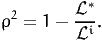
If some formulas have been requested to be reported, it is done in the next section. After is a list of statistics requested in the model specification file. The estimation report follows, including

• The number of parameters that have been estimated.
• The number of observations, that is, the number of rows in the data file that have not been excluded.
• The number of excluded observations.
• Init log likelihood is the log likelihood ⁱ of the sample for the model defined with the default values of the parameters.
• Final log likelihood is the log likelihood ^* of the sample for the estimated model.
• Likelihood ratio test for the init. model is

  (5)

  where ⁱ is the null log likelihood of the init model as defined above, and ^* is the log likelihood of the sample for the estimated model.

• Rho-square is

  (6)

• Rho-square-bar is

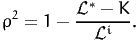  (7)

  where K is the number of estimated parameters. Note that this statistic is meaningless in the presence of constraints, where the number of degrees of freedom is less than the number of parameters.

• Final gradient norm is the gradient of the log likelihood function computed for the estimated parameters. If no constraint is active at the solution, it should be close to 0. If there are equality constraints, or if some bound constraints or inequality constraints are active at the solution (that is, they are verified with equality), the gradient may not be close to zero.
• Diagnostic is the diagnostic reported by the optimization algorithm. If the algorithm has not converged, the estimation results presented in the file cannot be used as such.
• Iterations is the number of iterations used by the algorithm before it stopped.
• Run time is the actual time used by the algorithm before it stopped, in minutes and seconds (format mm:ss).
• Nbr of thread: number of threads that is of processors, used during the estimation.

The following section reports the estimates of the parameters of the utility function, together with some statistics. For each parameter β_k, the following is reported:

• The name of the parameter.
• The estimated value β_k.
• The standard error σ_k of the estimate, calculated as the square root of the k^thdiagonal entry of the Rao-Cramer bound (see Appendix B).
• The t statistics, calculated as t_k = β_k∕σ_k.
• The p value, calculated as 2(1 - Φ(t_k)), where Φ(⋅) is the cumulative density function of the univariate standard normal distribution.
• A sign * is appended if the absolute value value of t_k is less than 1.96, emphasizing a potential lack of statistical significance. In this example, no such sign appears.
• The robust standard error σ_k^R of the estimate, calculated as the square root of the k^thdiagonal entry of the robust estimate of the variance covariance matrix. (see Appendix B).
• The robust t statistics, calculated as t_k^R = β_k∕σ_k^R.
• The robust p value, calculated as 2(1 - Φ(t_k^R)), where Φ(⋅) is the cumulative density function of the univariate normal distribution.
• A sign * is appended if the absolute value value of t_k^R is less than 1.96, emphasizing a potential lack of statistical significance. In this example, no such sign appears.

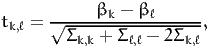
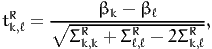
The last section reports, for each pair of parameters k and ℓ,

• the name of β_k,
• the name of β_ℓ,
• the entry Σ_k,ℓ of the Rao-Cramer bound (see Appendix B),
• the correlation between β_k and β_ℓ, calculated as

  (8)

• the t statistics, calculated as

  (9)

• a sign * is appended if the absolute value value of t_k,ℓ is less than 1.96, emphasizing that the hypothesis that the two parameters are equal cannot be rejected at the 5% level (in this example, no such sign appears),
• the entry Σ_k,ℓ^R of Σ^R, the robust estimate of the variance covariance matrix (see Appendix B),
• the robust correlation between β_k and β_ℓ, calculated as

  (10)

• the robust t statistics, calculated as

  (11)

• a sign * is appended if the absolute value value of t_k,ℓ^R is less than 1.96, emphasizing that the hypothesis that the two parameters are equal cannot be rejected at the 5% level (in this example, one such sign appears, for parameters B_COST and B_TIME).

The final line reports the value of the smallest singular value of the second derivatives matrix. A value close to zero is a sign of singularity, that may be due to a lack of variation in the data or an unidentified model.

A Complete specification file

A.1 01logit.py

B Estimation of the variance-covariance matrix

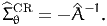
Under relatively general conditions, the asymptotic variance-covariance matrix of the maximum likelihood estimates of the vector of parameters θ ∈ℝ^K is given by the Cramer-Rao bound

(12)

The term in square brackets is the matrix of the second derivatives of the log likelihood function with respect to the parameters evaluated at the true parameters. Thus the entry in the kth row and the ℓth column is

(13)

Since we do not know the actual values of the parameters at which to evaluate the second derivatives, or the distribution of x_in and x_jn over which to take their expected value, we estimate the variance-covariance matrix by evaluating the second derivatives at the estimated parameters and the sample distribution of x_in and x_jn instead of their true distribution. Thus we use

(14)

as a consistent estimator of the matrix of second derivatives.

Denote this matrix as Â. Note that, from the second order optimality conditions of the optimization problem, this matrix is negative semi-definite, which is the algebraic equivalent of the local concavity of the log likelihood function. If the maximum is unique, the matrix is negative definite, and the function is locally strictly concave.

An estimate of the Cramer-Rao bound (12) is given by

(15)

If the matrix  is negative definite then - is invertible and the Cramer-Rao bound is positive definite.

Another consistent estimator of the (negative of the) second derivatives matrix can be obtained by the matrix of the cross-products of first derivatives as follows:

(16)

where

(17)

is the gradient vector of the likelihood of observation n. This approximation is employed by the BHHH algorithm, from the work by Berndt et al. (1974). Therefore, an estimate of the variance-covariance matrix is given by

(18)

although it is rarely used. Instead, is used to derive a third consistent estimator of the variance-covariance matrix of the parameters, defined as

(19)

It is called the robust estimator, or sometimes the sandwich estimator, due to the form of equation (19). Biogeme reports statistics based on both the Cramer-Rao estimate (15) and the robust estimate (19).

When the true likelihood function is maximized, these estimators are asymptotically equivalent, and the Cramer-Rao bound should be preferred (Kauermann and Carroll, 2001). When other consistent estimators are used, the robust estimator must be used (White, 1982). Consistent non-maximum likelihood estimators, known as pseudo maximum likelihood estimators, are often used when the true likelihood function is unknown or difficult to compute. In such cases, it is often possible to obtain consistent estimators by maximizing an objective function based on a simplified probability distribution.

References