Monte-Carlo integration with PythonBiogeme

Michel Bierlaire

August 6, 2015

Report TRANSP-OR 150806
Transport and Mobility Laboratory
School of Architecture, Civil and Environmental Engineering
Ecole Polytechnique Fédérale de Lausanne
transp-or.epfl.ch

Series on Biogeme

The package PythonBiogeme (biogeme.epfl.ch) is designed to estimate the parameters of various models using maximum likelihood estimation. It is particularly designed for discrete choice models. In this document, we investigate some aspects related to Monte-Carlo integration, which is particularly useful when estimating mixtures choice models, as well as choice models with latent variables. We assume that the reader is already familiar with discrete choice models, with PythonBiogeme, and with simulation methods, although a short summary is provided. This document has been written using PythonBiogeme 2.4, but should remain valid for future versions.

1 Monte-Carlo integration

Monte-Carlo integration consists in approximating an integral with the sum of a large number of terms. It comes from the definition of the expectation of a continuous random variable. Consider the random variable X with probability density function (pdf) fX(x). Assuming that X can take any value in the interval [a,b], where a {-} and b {+}, the expected value of X is given by

        ∫b
E [X ] =   xfX (x )dx.
         a
(1)

Also, if g : is a function, then

           ∫
            b
E [g (X)] =   g (x )fX (x )dx.
            a
(2)

The expectation of a random variable can be approximated using simulation. The idea is simple: generate a sample of realizations of X, that is generate R draws xr, r = 1,,R from X, and calculate the sample mean:

              R
           1-∑
E [g(X )] ≈ R    g (xr).
             r=1
(3)

Putting (2) and (3) together, we obtain an approximation to the integral:

∫ b               1 ∑R
   g(x)fX(x )dx  ≈ --    g(xr).
 a                R  r=1
(4)

Also, we have

∫
 b                     1-∑R
   g(x)fX(x)dx =  lRim→∞  R    g(xr).
 a                       r=1
(5)

Therefore, the procedure to calculate the following integral

    ∫b
I =    g(x)dx
     a
(6)

is the following

  1. Select a random variable X such that you can generate realizations of X, and such that the pdf fX is known;
  2. Generate R draws xr, r = 1,,R from X;
  3. Calculate
         1∑ R  g(x )
I ≈ --    ----r-.
    R  r=1 fX(xr)
    (7)

In order to obtain an estimate of the approximation error, we must calculate the variance the random variable. The sample variance is an unbiased estimate of the true variance:

             R
      --1---∑   g-(xr)     2
VR =  R - 1    (fX(xr) - I).
            r=1
(8)

Alternatively as

Var [g(X )] = E [g(X)2] - E [g(x)]2,
(9)

the variance can be approximated by simulation as well:

     1 ∑ R g (x )2
VR ≈ --    ----r- - I2.
     R  r=1 fX(xr)
(10)

Note that, for the values of R that we are using in this document, dividing by R or by R - 1 does not make much difference in practice. The approximation error is then estimated as

     ∘ ---
       Vr
eR =   ---.
        R
(11)

We refer the reader to Ross (2012) for a comprehensive introduction to simulation methods.

2 Uniform draws

There are many algorithms to draw from various distributions. All of them require at some point draws from the uniform distribution. There are several techniques that generate such uniform draws. In PythonBiogeme, one of them must be selected by setting the parameter RandomDistribution.

Each programming language provides a routine to draw a random number between 0 and 1. Such routines are deterministic, but the sequences of numbers that they generate share many properties with sequences of random numbers. Therefore, they are often called “pseudo random numbers”.

BIOGEME_OBJECT.PARAMETERS[RandomDistribution] = "PSEUDO"

Researchers have proposed to use other types of sequences to perform Monte-Carlo integration, called “quasi-random sequences” or “low-discrepancy sequences”. PythonBiogeme implements the Halton draws, from Halton (1960). They have been reported to perform well for discrete choice models (Train2000, Bhat2001, Bhat2003, Sándor and Train2004).

BIOGEME_OBJECT.PARAMETERS[RandomDistribution] = "HALTON"

The third method to generate uniform random numbers implemented in PythonBiogeme is called “Modified Latin Hypercube Sampling”, and has been proposed by Hess et al. (2006).

BIOGEME_OBJECT.PARAMETERS[RandomDistribution] = "MHLS"

In the following, we are using these three options, and compare the accuracy of the corresponding Monte-Carlo integration.

3 Illustration with PythonBiogeme

We first illustrate the method on a simple integral. Consider

    ∫1
        x
I =  0 e dx.
(12)

In this case, it can be solved analytically:

I = e - 1 = 1. 7183.
(13)

In order to use Monte-Carlo integration, we consider the random variable X that is uniformly distributed on [0,1], so that

        {
f (x) =    1  if x ∈ [0, 1],
 X         0  otherwise.
(14)

Therefore, we can approximate I by generating R draws from X and

               R     x        R
I = E[eX] ≈ 1-∑   -e-r-- = 1-∑   exr.
            R     fX(xr)   R
              r=1             r=1
(15)

Moreover, as

Var[eX] = E[e2X] - E [eX]2
          ∫1
       =    e2xdx - (e - 1)2
           0
       =  (e2 - 1 )∕2 - (e - 1)2

       =  0. 2420356075,
(16)

the standard error is 0.0034787613 for R = 20000, and 0.0011000809 for R = 200000. These theoretical values are estimated also below using PythonBiogeme.

We use PythonBiogeme to calculate (15). Note that PythonBiogeme requires a data file, which is not necessary in this simplistic case. We use the simulation mode of PythonBiogeme. It generates output for each row of the data file. In our case, we just need one output, so that we take any data file, and exclude all rows of the file except the first one, using the following syntax:

__rowId__ = Variable(__rowId__) 
BIOGEME_OBJECT.EXCLUDE = __rowId__ >= 1

For this specific example, the data included in the file are irrelevant. The generation of draws in PythonBiogeme is performed using the command bioDraws(U), where the argument U provides the name of the random variable associated with the draws. The distribution of the random variable is specified using the following syntax:

BIOGEME_OBJECT.DRAWS = { U: UNIFORM}

Note that the valid keywords are

The integrand is defined by the following statement:

integrand = exp(bioDraws(U))

and the Monte-Carlo integration is obtained as follows:

simulatedI = MonteCarlo(integrand)

The number of draws is defined by the parameter NbrOfDraws:

BIOGEME_OBJECT.PARAMETERS[NbrOfDraws] = "20000"

We calculate as well the simulated variance, using (10):

sampleVariance = \ 
  MonteCarlo(integrand*integrand) - simulatedI * simulatedI

and the standard error (11):

stderr = (sampleVariance / 20000.0)**0.5

Also, as we know the true value of the integral

trueI = exp(1.0) - 1.0

we can calculate the error:

error = simulatedI - trueI

The calculation is obtained using the following statements:

simulate = {01 Simulated Integral: simulatedI, 
            02 Analytical Integral: trueI, 
            03 Sample variance: sampleVariance, 
            04 Std Error: stderr, 
            05 Error: error} 
 
rowIterator(obsIter) 
 
BIOGEME_OBJECT.SIMULATE = Enumerate(simulate,obsIter)

We obtain the following results:

Simulated Integral 1.72007
Analytical Integral 1.71828
Sample variance 0.240135
Std Error 0.00346508
Error 0.00178739

Remember that the true variance is 0.2420356075, and the true standard error is 0.0034787613. If we use ten times more draws, that is 200,000 draws, we obtain a more precise value:

Simulated Integral 1.71902
Analytical Integral 1.71828
Sample variance 0.24175
Std Error 0.00109943
Error 0.000739329

Remember that the true variance is 0.2420356075, and the true standard error is 0.0011000809. The complete specification file for PythonBiogeme is available in Appendix A.1.

4 Variance reduction

There are several techniques to reduce the variance of the draws used for the Monte-Carlo integration. Reducing the variance improves the precision of the approximation for the same number of draws. Equivalently, they allow to use less draws to achieve the same precision. We introduce two of them in this document: antithetic draws, and control variates. As the focus of this document is on PythonBiogeme, we urge the reader to read an introduction to variance reduction methods in simulation, for instance in Ross (2012).

4.1 Antithetic draws

Instead of drawing from X, consider two random variables X1 and X2, identically distributed with pdf fX = fX1 = fX2, and define a new random variable

Y = X1-+-X2-.
       2
(17)

Then, as E[Y] = E[X1] = E[X2] = E[X], we can rewrite (1) as follows:

                                  ∫
       1-        1-                 b
E[Y] = 2 E[X1] + 2 E[X2] = E[X ] =   xfX(x)dx.
                                   a
(18)

The variance of this quantity is

         1-
Var[Y] = 4(Var (X1) + Var(X2) + 2Cov (X1, X2)).
(19)

If X1 and X2 are independent, this variance is equal to

Var[Y ] = 1-Var [X ].
         2
(20)

Therefore, using Y for Monte-Carlo integration is associated with a variance divided by two, but requires twice more draws (R draws for X1 and R draws for X2). It has no advantage on drawing directly R draws from X. Formally, we can compare the standard errors of the two methods for the same number of draws. Drawing 2R draws from X, we obtain the following standard error:

∘ -------
   Var[X]-
     2R  .
(21)

Drawing R draws from X1 and R draws from X2 to generate R draws from Y, we obtain the same standard error

∘  -------  ∘ -------
   Var[Y]      Var[X]
   -------=    ------.
     R           2R
(22)

However, if the variables X1 and X2 happen to be negatively correlated, that is if Cov(X1,X2) < 0, then Var[Y] < Var[X]∕2, and drawing from Y reduces the standard error. For instance, if X1 is uniformly distributed on [0,1], then X2 = 1 - X1 is also uniformly distributed on [0,1], and

                                                   1
Cov (X1, X2) = E[X1(1 - X1 )] - E[X1]E [1 - X1 ] = ----<  0.
                                                  12
(23)

If X1 has a standard normal distribution, that is such that E[X1] = 0 and Var[X1] = 1, then X2 = -X1 has also a standard normal distribution, and is negatively correlated with X1, as

Cov (X1, X2) = E[-X21] - E[X1]E [-X1 ] = -1 <  0.
(24)

The other advantage of this method is that we can recycle the draws. Once we have generated the draws xr from X1, the draws from X2 are obtained using 1 - xr and -xr, respectively.

Now, we have to be careful when this technique is used for the general case (2). Indeed, it must be verified first that g(X1) and g(X2) are indeed negatively correlated. And it is not guaranteed by the fact that X1 and X2 are negatively correlated. Consider two examples.

First, consider g(X) = (      )
 x -  122. Applying the antithetic method with

     (       )2           (             )2
X1 =   X -  1-   and X2 =   (1 - X) - 1-
            2                         2
(25)

does not work, as

Cov (X1, X2) = -1-->  0.
               180
(26)

Actually, applying the antithetic method would increase the variance here, which is not desirable.

Second, consider g(X) = eX, as in the example presented in Section 3. We apply the antithetic method using

     X    1-X
Y = e--+-e----.
        2
(27)

Here, the two transformed random variables are negatively correlated:

      X  1-X       X 1-X       X     1-X
Cov (e , e  ) = E[e e   ] - E[e ]E [e    ]
              = e - (e - 1)2

              = -0. 2342106136.
(28)

Therefore, the variance of Y given by (19) is 0.0039124969, as opposed to 0.2420356075∕2 = 0.1210178037 if the two sets of draws were independent. It means that for 10000 draws from Y, the standard error decreases from 0.0034787613 down to 0.0006254996. Moreover, as we use recycled draws, we need only 10000 draws instead of 20000.

To apply this technique in PythonBiogeme, the integrand is defined as follows:

integrand = 0.5 * (exp(bioDraws(U)) + exp(1.0-bioDraws(U)))

and the number of draws reduced to 10000:

stderr = (sampleVariance / 10000.0)**0.5 
BIOGEME_OBJECT.PARAMETERS[NbrOfDraws] = "10000"

We obtain the following results:

Simulated Integral 1.71708
Analytical Integral 1.71828
Sample variance 0.00380337
Std Error 0.000616715
Error -0.00120542

The reader can compare these values with the theoretical derivation presented above. The complete specification file for PythonBiogeme is available in Appendix A.2.

4.2 Control variate

The control variate method reduces the variance by exploiting information from another random variable, correlated with g(X), with a known mean. Consider the random variable Y such that E[Y] = μ. We define a new random variable Z as follows:

Z = g (X) + c(Y - μ)
(29)

where c is a parameter. By construction, E[Z] = E[g(X)] for any c, so that draws from Z can be used instead of draws from g(X) for Monte-Carlo integration. Note that we do not need any assumption on g here. The idea is to identify the value of c that minimizes the variance of Z. We have

Var[Z ] = Var [g (X) + cY] = Var[g(X )] + c2Var [Y ] + 2c Cov (g(X), Y ),
(30)

which is minimized for

       Cov (g(X), Y )
c* = - -------------.
          Var[Y ]
(31)

Therefore, we use for Monte-Carlo integration the random variable
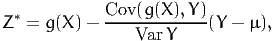
Z * = g(X) - Cov-(g(X-), Y-)(Y - μ),
                 Var Y
(32)

with variance

                                    2
Var [Z *] = Var[g(X)] - Cov-(g(X), Y-)-≤ Var[g(X )].
                           Var Y
(33)

Note that, as for antithetic draws, this technique exploits the correlation between two random variables. If Y is independent from g(X), no variance reduction is achieved.

In our example, g(X) = eX. If we select Y = X, we know that

       1                1
E[Y] = --and  Var[Y] = ---.
       2               12
(34)

Moreover,

                      X
Cov (g (X ), Y) = Cov (e , X ) = (3 - e )∕2 = 0.1408590858.
(35)

Therefore, we obtain

  *    Cov-(g-(X-), Y)
c  = -     Var Y     = -6 (3 - e) = -1. 6903090292,
(36)

and the variance of Z* is 0.0039402229, which is much lower than the variance of x, that is 0.2420356075. It means that, for 20000 draws, the standard error is 0.0004438594, as opposed to 0.0034787613. With this method, only 326 draws are sufficient to achieve the same precision as the Monte-Carlo integration without control variate. Indeed,

∘ --------------
   0.0039402229---
        326      = 0. 003476575.
(37)

This is a tremendous saving. The control variate method is invoked in PythonBiogeme using the following statement:

simulatedI = MonteCarloControlVariate(integrand,bioDraws(U),0.5),

where the second argument bioDraws(U) is Y, and the third, 0.5, is μ. Note that, in addition to the output requested by the user, PythonBiogeme also generates a report containing statistics on g(X), Y and Z*. In particular, it reports both the simulated value of Y and μ to detect any implementation error.

The results of the Monte-Carlo integration are:

Simulated Integral (E[Z*]) 1.71759
Simulated Integral (E[X]) 1.72007
Analytical Integral 1.71828
Sample variance (Var[X]) 0.239849
Std Error (∘ ---------------
  Var[Z *]∕20000) 0.000440564
Error -0.00069233

The complete specification file for PythonBiogeme is available in Appendix A.3.

Finally, we present in Table 1 the results of the three methods, using different types of uniform draws as described in Section 2. For each technique, the standard errors for the three types of draws are comparable, with the antithetic draws achieving the best value, followed by the control variate. However, the precision actually achieved is much better for Halton, and even more for MLHS.


Pseudo
Halton
MHLS


Monte-Carlo 1.71902 1.71814 1.71829
Standard error 0.00109943 0.00109999 0.00110009
Actual error 0.000739329 -0.000145885 9.38555e-06


Antithetic 1.71708 1.71828 1.71828
Standard error 0.000616715 0.000625455 0.0006255
Actual error -0.00120542 -2.27865e-06 -6.13416e-10


Control variate 1.71759 1.71828 1.71828
Standard error 0.000440564 0.000443827 0.000443872
Actual error -0.00069233 -2.84647e-06 1.52591e-07


Table 1: Comparison of variants of Monte-Carlo integration on the simple example

We encourage the reader to perform similar tests for other simple integrals. For instance,

∫1(     1)2        1
    x - --  dx =  ---
 0      2         12
(38)

or

∫2 (                )
     e-x + ----1----  dx  = e2 - e-2 + log 4-+-ε,
 -2        2 + ε - x                        ε
(39)

where ε > 0. Note that the domain of integration is not [0,1].

5 Mixtures of logit

Consider an individual n, a choice set Cn, and an alternative i Cn. The probability to choose i is given by the choice model:

Pn(i|x, θ, Cn),
(40)

where x is a vector of explanatory variables and θ is a vector of parameters to be estimated from data. In the random utility framework, a utility function is defined for each individual n and each alternative i Cn:

Uin (x, θ) = Vin(x, θ ) + εin(θ),
(41)

where Vin(x,θ) is deterministic and εin is a random variable independent from x. The model is then written:

Pn(i|x, θ, Cn) = Pr(Uin (x, θ) ≥ Ujn(x, θ), ∀j ∈ Cn).
(42)

Specific models are obtained from assumptions about the distribution of εin. Namely, if εin are i.i.d. (across both i and n) extreme value distributed, we obtain the logit model:

                   eVin(x,θ)
Pn (i|x, θ, Cn ) = ∑----V--(x,θ).
                  j∈Cn e jn
(43)

Mixtures of logit are obtained when some of the parameters θ are distributed instead of being fixed. Denote θ = (θfd), where θf is the vector of fixed parameters, while θd is the vector of distributed parameters, so that the choice model, conditional on θd, is

P (i|x, θ , θ , C ).
 n      f  d  n
(44)

A distribution is to be assumed for θd. We denote the pdf of this distribution by fθd(ξ;γ), where γ contains the parameters of the distribution. Parameters γ are sometimes called the deep parameters of the model. Therefore, the choice model becomes:

                   ∫
Pn (i|x, θf, γ, Cn) = Pn (i|x, θf, ξ, Cn )fθ (ξ)d ξ,
                    ξ                 d
(45)

where θf and γ must be estimated from data. The above integral has no analytical solution, even when the kernel Pn(i|x,θf,ξ,Cn) is a logit model. Therefore, it must be calculated with numerical integration or Monte-Carlo integration. We do both here to investigate the precision of the variants of Monte-Carlo integration.

5.1 Comparison of integration methods on one integral

We consider the Swissmetro example (Bierlaire et al.2001). The data file is available from biogeme.epfl.ch. Consider the following specification:

As there is only one random parameter, the model (45) can be calculated using numerical integration. It is done in PythonBiogeme using the following procedure:

  1. Mention that omega is a random variable:
    omega = RandomVariable(omega)
  2. Define its pdf:
    density = normalpdf(omega).

    Make sure that the library distributions is loaded in order to use the function normalpdf, using the following statement:

    from distributions import *
  3. Define the integrand from the logit model, where the probability of the alternative observed to be chosen is calculated (which is typical when calculating a likelihood function):
    integrand = bioLogit(V,av,CHOICE)
  4. Calculate the integral:
    analyticalI = Integrate(integrand*density,omega)

The complete specification file for PythonBiogeme is available in Appendix A.4. The value of the choice model for first observation in the data file is
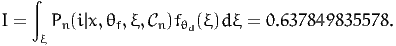
    ∫
I =    P (i|x, θ , ξ, C )f (ξ)dξ = 0.637849835578.
     ξ  n      f    n  θd
(46)

Note that, in order ot obtain so many significant digits, we have used the following statement:

BIOGEME_OBJECT.PARAMETERS[decimalPrecisionForSimulation] = "12"

To calculate the same integral with Monte-Carlo integration, we use the same syntax as described earlier in this document:

omega = bioDraws(B_TIME_RND) 
BIOGEME_OBJECT.PARAMETERS[NbrOfDraws] = "20000" 
BIOGEME_OBJECT.DRAWS = { B_TIME_RND: NORMAL } 
B_TIME_RND = B_TIME + B_TIME_S * omega 
integrand = bioLogit(V,av,CHOICE) 
simulatedI = MonteCarlo(integrand)

The complete specification file for PythonBiogeme is available in Appendix A.5. Using the result of the numerical integration as the “true” value of the integral, We obtain the following results:

Simulated integral 0.637263
Numerical integration 0.63785
Sample variance 0.0299885
Std Error 0.000387224
Error -0.000586483

We now apply the variance reduction methods. The antithetic draws described in Section 4.1 are generated as follows:

  1. As we are dealing with draws from the normal distribution, the antithetic draw of xr is -xr. We create two versions of the parameter, one with the draw, and one with its antithetic:
    B_TIME_RND = B_TIME + B_TIME_S * bioDraws(B_TIME_RND) 
    B_TIME_RND_MINUS = B_TIME - B_TIME_S * bioDraws(B_TIME_RND)
  2. Consistently, we then generate two versions of the model:
    V1_MINUS = ASC_TRAIN + \ 
               B_TIME_RND_MINUS * TRAIN_TT_SCALED + \ 
               B_COST * TRAIN_COST_SCALED 
    V2_MINUS = ASC_SM + \ 
               B_TIME_RND_MINUS * SM_TT_SCALED + \ 
               B_COST * SM_COST_SCALED 
    V3_MINUS = ASC_CAR + \ 
               B_TIME_RND_MINUS * CAR_TT_SCALED + \ 
               B_COST * CAR_CO_SCALED 
    V_MINUS = {1: V1_MINUS, 
               2: V2_MINUS, 
               3: V3_MINUS}
  3. The integrand is the average of the integrands generated by the two versions of the model:
    integrand_plus = bioLogit(V,av,CHOICE) 
    integrand_minus = bioLogit(V_MINUS,av,CHOICE) 
    integrand = 0.5 * (integrand_plus + integrand_minus)

The complete specification file for PythonBiogeme is available in Appendix A.6.

The control variate method, described in Section 4.2, requires an output of the simulation such that the analytical integral is known. We propose here to consider
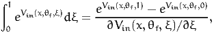
∫
 1 V  (x,θ,ξ)      eVin(x,θf,1) - eVin(x,θf,0)
  e in  f  dξ =  ---------------------,
 0                 ∂Vin(x, θf, ξ)∕∂ξ
(47)

if ∂Vin(x,θf)∕∂ξ does not depend on ξ. This integral is calculated by Monte-Carlo after recycling the uniform draws used to generate the normal draws for the original integration. We follow the following procedure:

  1. We recycle the draws:
    UNIFDRAW = bioRecycleDraws(B_TIME_RND)
  2. We calculate the control variate integrand:
    VCV = ASC_TRAIN + \ 
          (B_TIME + B_TIME_S * UNIFDRAW) * TRAIN_TT_SCALED + \ 
          B_COST * TRAIN_COST_SCALED

    Note that the derivative with respect to UNIFDRAW is

    B_TIME_S * TRAIN_TT_SCALED$.
  3. We provide the analytical value of the control variate integral:
    VCV_ZERO = ASC_TRAIN + \ 
               B_TIME * TRAIN_TT_SCALED + \ 
               B_COST * TRAIN_COST_SCALED 
    VCV_ONE = ASC_TRAIN + \ 
             (B_TIME + B_TIME_S ) * TRAIN_TT_SCALED + \ 
             B_COST * TRAIN_COST_SCALED 
    VCV_INTEGRAL = (exp(VCV_ONE) - exp(VCV_ZERO)) / \ 
                   (B_TIME_S * TRAIN_TT_SCALED)
  4. We perform the Monte-Carlo integration:
    simulatedI = MonteCarloControlVariate(integrand,\ 
                                          exp(VCV),\ 
                                          VCV_INTEGRAL)

The complete specification file for PythonBiogeme is available in Appendix A.7.

Table 2 provides the results of the Monte-Carlo integration using different variance reduction methods (none, antithetic and control variates), different uniform draws (pseudo, Halton and MLHS), and different number of draws.

We can observe the following:

It would be useful to perform the same experiment for some other observations in the data file. Such experiments can give useful insights to for the choice of the most appropriate integration technique. In the following, we compare some of these techniques for the maximum likelihood estimation of the parameters of the model.


20000 draws
2000 draws
500 draws
Draws
Pseudo
Halton
MHLS


Monte-Carlo 20000 0.637263 0.637923 0.637845
Standard error 0.000387224 0.000390176 0.000390301
Actual error -0.000586483 7.35443e-05 -5.08236e-06


Antithetic 10000 0.638383 0.637856 0.63785
Standard error 5.13243e-05 5.24484e-05 5.24949e-05
Actual error 0.000533174 6.1286e-06 1.96217e-07


Control variate 20000 0.6377 0.637871 0.637848
Standard error 0.000176759 0.000179054 0.00017928
Actual error -0.000149889 2.127e-05 -1.72413e-06


Antithetic 1000 0.638783 0.637965 0.637853
Standard error 5.05914e-05 5.17454e-05 5.24619e-05
Actual error 0.000933592 0.000114998 3.32666e-06


Control variate 2000 0.637876 0.637975 0.637835
Standard error 0.000551831 0.00056032 0.000567009
Actual error 2.66122e-05 0.000125218 -1.50796e-05


Antithetic 250 0.639205 0.638459 0.637869
Standard error 5.17638e-05 4.97379e-05 5.23141e-05
Actual error 0.00135483 0.000609069 1.87082e-05


Control variate 500 0.637587 0.638158 0.637798
Standard error 0.00111188 0.00109022 0.00113287
Actual error -0.000262395 0.000308626 -5.2274e-05


Table 2: Comparison of variants of Monte-Carlo integration on the mixture of logit example

5.2 Comparison of integration methods for maximum likelihood estimation

We now estimate the parameters of the model using all observations in the data set associated with work trips. Observations such that the dependent variable CHOICE is 0 are also removed.

exclude = (( PURPOSE != 1 ) * (  PURPOSE   !=  3  ) + \ 
          ( CHOICE == 0 )) > 0 
BIOGEME_OBJECT.EXCLUDE = exclude

The estimation using numerical integration is performed using the following statements:

integrand = bioLogit(V,av,CHOICE) 
prob = Integrate(integrand*density,omega) 
l = log(prob) 
rowIterator(obsIter) 
BIOGEME_OBJECT.ESTIMATE = Sum(l,obsIter)

The complete specification file for PythonBiogeme is available in Appendix A.8.

For Monte-Carlo integration, we use the following statements:

prob = bioLogit(V,av,CHOICE) 
l = mixedloglikelihood(prob) 
rowIterator(obsIter) 
BIOGEME_OBJECT.ESTIMATE = Sum(l,obsIter)

where the statement l = mixedloglikelihood(prob) is equivalent to

integral = MonteCarlo(prob) 
l = log(integral)

The complete specification file for PythonBiogeme is available in Appendix A.9.

The following estimation results are presented:

The final log likelihood in each case, as well as the estimation time are summarized in Table 3. In this experiment, when looking at the estimates, it seems that the MLHS draws provide relatively good precision, even for a lower number of draws, and with no variance reduction. Clearly, this result cannot be generalized, and should be investigated on a case by case basis. Note however that the default type of draws in PythonBiogeme is MLHS, because it is performing particularly well in this example.


Method Draws Log likelihood Run time


Numerical -5214.879 02:37
Monte-Carlo 2000 -5214.835 31:11
Antithetic 1000 -5214.899 39:26
Control variate 2000 -5214.835 42:11
Monte-Carlo 500 -5214.940 09:26
Antithetic 250 -5214.897 09:21
Control variate 500 -5214.940 08:59

Table 3: Final log likelihood and run time for each integration method


Robust
Parameter
Coeff.
Asympt.
numberDescription
estimate
std. error
t-stat
p-value


1

ASC_CAR

0. 137 0. 0517 2. 65 0. 01
2

ASC_TRAIN

-0. 401 0. 0656 -6. 12 0. 00
3

B_COST

-1. 29 0. 0863 -14. 90 0. 00
4

B_TIME

-2. 26 0. 117 -19. 38 0. 00
5

B_TIME_S

-1. 65 0. 125 -13. 26 0. 00


Summary statistics
Number of observations = 6768
Number of excluded observations = 3960
Number of estimated parameters = 5
Number of iterations = 13
Estimation time: 00 : 02 : 37
L(β0)=-7157.671
L(^
β)=-5214.879
-2[L(β0) - L(^
β)]=3885.585
ρ2=0.271
ρ2=0.271

Table 4: Estimation results with numerical integration


Robust
Parameter
Coeff.
Asympt.
numberDescription
estimate
std. error
t-stat
p-value


1

ASC_CAR

0. 137 0. 0517 2. 65 0. 01
2

ASC_TRAIN

-0. 402 0. 0658 -6. 10 0. 00
3

B_COST

-1. 29 0. 0864 -14. 89 0. 00
4

B_TIME

-2. 26 0. 117 -19. 31 0. 00
5

B_TIME_S

1. 66 0. 132 12. 59 0. 00


Summary statistics
Number of observations = 6768
Number of excluded observations = 3960
Number of estimated parameters = 5
Number of iterations = 9
Estimation time: 00 : 31 : 11
L(β0)=-6964.663
L(^
β)=-5214.835
-2[L(β0) - L(^
β)]=3499.656
ρ2=0.251
ρ2=0.251

Table 5: Estimation results with Monte-Carlo, no variance reduction, 2000 MHLS draws


Robust
Parameter
Coeff.
Asympt.
numberDescription
estimate
std. error
t-stat
p-value


1

ASC_CAR

0. 137 0. 0517 2. 65 0. 01
2

ASC_TRAIN

-0. 402 0. 0658 -6. 10 0. 00
3

B_COST

-1. 29 0. 0863 -14. 89 0. 00
4

B_TIME

-2. 26 0. 117 -19. 31 0. 00
5

B_TIME_S

1. 66 0. 132 12. 59 0. 00


Summary statistics
Number of observations = 6768
Number of excluded observations = 3960
Number of estimated parameters = 5
Number of iterations = 12
Estimation time: 00 : 39 : 26
L(β0)=-7155.875
L(^
β)=-5214.899
-2[L(β0) - L(^
β)]=3881.952
ρ2=0.271
ρ2=0.271

Table 6: Estimation results with antithetic draws, 1000 MHLS draws


Robust
Parameter
Coeff.
Asympt.
numberDescription
estimate
std. error
t-stat
p-value


1

ASC_CAR

0. 137 0. 0517 2. 65 0. 01
2

ASC_TRAIN

-0. 402 0. 0658 -6. 10 0. 00
3

B_COST

-1. 29 0. 0864 -14. 89 0. 00
4

B_TIME

-2. 26 0. 117 -19. 31 0. 00
5

B_TIME_S

1. 66 0. 132 12. 59 0. 00


Summary statistics
Number of observations = 6768
Number of excluded observations = 3960
Number of estimated parameters = 5
Number of iterations = 12
Estimation time: 00 : 42 : 11
L(β0)=-7155.867
L(^
β)=-5214.835
-2[L(β0) - L(^
β)]=3882.063
ρ2=0.271
ρ2=0.271

Table 7: Estimation results with control variates, 2000 MHLS draws


Robust
Parameter
Coeff.
Asympt.
numberDescription
estimate
std. error
t-stat
p-value


1

ASC_CAR

0. 137 0. 0517 2. 65 0. 01
2

ASC_TRAIN

-0. 402 0. 0658 -6. 10 0. 00
3

B_COST

-1. 29 0. 0864 -14. 88 0. 00
4

B_TIME

-2. 26 0. 117 -19. 33 0. 00
5

B_TIME_S

1. 66 0. 131 12. 63 0. 00


Summary statistics
Number of observations = 6768
Number of excluded observations = 3960
Number of estimated parameters = 5
Number of iterations = 12
Estimation time: 00 : 09 : 26
L(β0)=-7155.962
L(^
β)=-5214.940
-2[L(β0) - L(^
β)]=3882.044
ρ2=0.271
ρ2=0.271

Table 8: Estimation results with Monte-Carlo integration, no variance reduction, 500 MHLS draws


Robust
Parameter
Coeff.
Asympt.
numberDescription
estimate
std. error
t-stat
p-value


1

ASC_CAR

0. 137 0. 0517 2. 65 0. 01
2

ASC_TRAIN

-0. 402 0. 0658 -6. 11 0. 00
3

B_COST

-1. 29 0. 0864 -14. 88 0. 00
4

B_TIME

-2. 26 0. 117 -19. 33 0. 00
5

B_TIME_S

1. 66 0. 131 12. 61 0. 00


Summary statistics
Number of observations = 6768
Number of excluded observations = 3960
Number of estimated parameters = 5
Number of iterations = 12
Estimation time: 00 : 09 : 21
L(β0)=-7155.877
L(^
β)=-5214.897
-2[L(β0) - L(^
β)]=3881.960
ρ2=0.271
ρ2=0.271

Table 9: Estimation results with antithetic draws, 250 MHLS draws


Robust
Parameter
Coeff.
Asympt.
numberDescription
estimate
std. error
t-stat
p-value


1

ASC_CAR

0. 137 0. 0517 2. 65 0. 01
2

ASC_TRAIN

-0. 402 0. 0658 -6. 10 0. 00
3

B_COST

-1. 29 0. 0864 -14. 88 0. 00
4

B_TIME

-2. 26 0. 117 -19. 33 0. 00
5

B_TIME_S

1. 66 0. 131 12. 63 0. 00


Summary statistics
Number of observations = 6768
Number of excluded observations = 3960
Number of estimated parameters = 5
Number of iterations = 12
Estimation time: 00 : 08 : 59
L(β0)=-7155.962
L(^
β)=-5214.940
-2[L(β0) - L(^
β)]=3882.044
ρ2=0.271
ρ2=0.271

Table 10: Estimation results with control variates, 500 MHLS draws

6 Conclusion

This document describes the variants of Monte-Carlo integration, and suggests how to perform some analysis using the SIMULATE operator of PythonBiogeme, that helps investigating the performance of each of them before starting a maximum likelihod estimation, that may take a while to converge. In the example provided in this document, the antithetic draws method, combined with MLHS appeared to be the most precise. This result is not universal. The analysis must be performed on a case by case basis.

A Complete specification files

A.1 01simpleIntegral.py

 
1####################################### 
2# 
3# File: 01simpleIntegral.py 
4# Author: Michel Bierlaire, EPFL 
5# Date: Sat Jul 25 11:41:13 2015 
6# 
7####################################### 
8 
9from biogeme import * 
10from headers import * 
11 
12integrand = exp(bioDraws(U)) 
13simulatedI = MonteCarlo(integrand) 
14 
15trueI = exp(1.0) - 1.0 
16 
17sampleVariance = \ 
18  MonteCarlo(integrand*integrand) - simulatedI * simulatedI 
19stderr = (sampleVariance / 200000.0)**0.5 
20error = simulatedI - trueI 
21 
22simulate = {01 Simulated Integral: simulatedI, 
23            02 Analytical Integral: trueI, 
24            03 Sample variance: sampleVariance, 
25            04 Std Error: stderr, 
26            05 Error: error} 
27 
28rowIterator(obsIter) 
29 
30BIOGEME_OBJECT.SIMULATE = Enumerate(simulate,obsIter) 
31BIOGEME_OBJECT.PARAMETERS[NbrOfDraws] = "5" 
32BIOGEME_OBJECT.PARAMETERS[RandomDistribution] = "PSEUDO" 
33__rowId__ = Variable(__rowId__) 
34BIOGEME_OBJECT.EXCLUDE = __rowId__ >= 1 
35BIOGEME_OBJECT.DRAWS = { U: UNIFORM}

A.2 02antithetic.py

 
1####################################### 
2# 
3# File: 02antithetic.py 
4# Author: Michel Bierlaire, EPFL 
5# Date: Sat Jul 25 12:21:10 2015 
6# 
7####################################### 
8 
9from biogeme import * 
10from headers import * 
11 
12integrand = 0.5 * (exp(bioDraws(U)) + exp(1.0-bioDraws(U))) 
13simulatedI = MonteCarlo(integrand) 
14 
15trueI = exp(1.0) - 1.0 
16 
17sampleVariance = \ 
18  MonteCarlo(integrand*integrand) - simulatedI * simulatedI 
19stderr = (sampleVariance / 10000.0)**0.5 
20error = simulatedI - trueI 
21 
22simulate = {01_Simulated Integral: simulatedI, 
23            02_Analytical Integral: trueI, 
24            03_Sample variance: sampleVariance, 
25            04_Std Error: stderr, 
26            05_Error: error} 
27 
28rowIterator(obsIter) 
29 
30BIOGEME_OBJECT.SIMULATE = Enumerate(simulate,obsIter) 
31 
32BIOGEME_OBJECT.PARAMETERS[NbrOfDraws] = "5" 
33__rowId__ = Variable(__rowId__) 
34BIOGEME_OBJECT.EXCLUDE = __rowId__ >= 1 
35BIOGEME_OBJECT.DRAWS = { U: UNIFORM}

A.3 03controlVariate.py

 
1####################################### 
2# 
3# File: 03controlVariate.py 
4# Author: Michel Bierlaire, EPFL 
5# Date: Sat Jul 25 12:24:25 2015 
6# 
7####################################### 
8# 
9 
10from biogeme import * 
11from headers import * 
12 
13integrand = exp(bioDraws(U)) 
14simulatedI = MonteCarloControlVariate(integrand,bioDraws(U),0.5) 
15 
16trueI = exp(1.0) - 1.0 
17 
18error = simulatedI - trueI 
19 
20simulate = {01_Simulated Integral: simulatedI, 
21            02_Analytical Integral: trueI, 
22            05_Error: error} 
23 
24rowIterator(obsIter) 
25 
26BIOGEME_OBJECT.SIMULATE = Enumerate(simulate,obsIter) 
27 
28BIOGEME_OBJECT.PARAMETERS[NbrOfDraws] = "5" 
29__rowId__ = Variable(__rowId__) 
30BIOGEME_OBJECT.EXCLUDE = __rowId__ >= 1 
31BIOGEME_OBJECT.DRAWS = { U: UNIFORM}

A.4 05normalMixtureTrueAnalytical.py

 
1####################################### 
2# 
3# File: 05normalMixtureTrueAnalytical.py 
4# Author: Michel Bierlaire, EPFL 
5# Date: Sat Jul 25 18:50:11 2015 
6# 
7####################################### 
8 
9from biogeme import * 
10from headers import * 
11from distributions import * 
12from loglikelihood import * 
13 
14#Parameters 
15ASC_CAR = 0.137 
16ASC_TRAIN = -0.402 
17ASC_SM = 0 
18B_TIME = -2.26 
19B_TIME_S = 1.66 
20B_COST = -1.29 
21 
22# Define a random parameter, normally distributed, 
23# designed to be used for integration 
24omega = RandomVariable(omega) 
25density = normalpdf(omega) 
26B_TIME_RND = B_TIME + B_TIME_S * omega 
27 
28# Utility functions 
29 
30#If the person has a GA (season ticket) her 
31#incremental cost is actually 0 
32#rather than the cost value gathered from the 
33# network data. 
34SM_COST =  SM_CO   * (  GA   ==  0  ) 
35TRAIN_COST =  TRAIN_CO   * (  GA   ==  0  ) 
36 
37# For numerical reasons, it is good practice to scale the data to 
38# that the values of the parameters are around 1.0. 
39# A previous estimation with the unscaled data has generated 
40# parameters around -0.01 for both cost and time. 
41# Therefore, time and cost are multipled my 0.01. 
42 
43TRAIN_TT_SCALED = \ 
44  DefineVariable(TRAIN_TT_SCALED, TRAIN_TT / 100.0) 
45TRAIN_COST_SCALED = \ 
46  DefineVariable(TRAIN_COST_SCALED, TRAIN_COST / 100) 
47SM_TT_SCALED = DefineVariable(SM_TT_SCALED, SM_TT / 100.0) 
48SM_COST_SCALED = DefineVariable(SM_COST_SCALED, SM_COST / 100) 
49CAR_TT_SCALED = DefineVariable(CAR_TT_SCALED, CAR_TT / 100) 
50CAR_CO_SCALED = DefineVariable(CAR_CO_SCALED, CAR_CO / 100) 
51 
52V1 = ASC_TRAIN + \ 
53     B_TIME_RND * TRAIN_TT_SCALED + \ 
54     B_COST * TRAIN_COST_SCALED 
55V2 = ASC_SM + \ 
56     B_TIME_RND * SM_TT_SCALED + \ 
57     B_COST * SM_COST_SCALED 
58V3 = ASC_CAR + \ 
59     B_TIME_RND * CAR_TT_SCALED + \ 
60     B_COST * CAR_CO_SCALED 
61 
62 
63# Associate utility functions with the numbering of alternatives 
64V = {1: V1, 
65     2: V2, 
66     3: V3} 
67 
68# Associate the availability conditions with the alternatives 
69 
70CAR_AV_SP =  DefineVariable(CAR_AV_SP,CAR_AV  * (  SP   !=  0  )) 
71TRAIN_AV_SP =  DefineVariable(TRAIN_AV_SP,TRAIN_AV  * (  SP   !=  0  )) 
72 
73av = {1: TRAIN_AV_SP, 
74      2: SM_AV, 
75      3: CAR_AV_SP} 
76 
77# The choice model is a logit, with availability conditions 
78integrand = bioLogit(V,av,CHOICE) 
79 
80 
81analyticalI = Integrate(integrand*density,omega) 
82simulate = {Analytical: analyticalI} 
83 
84rowIterator(obsIter) 
85 
86BIOGEME_OBJECT.PARAMETERS[decimalPrecisionForSimulation] = "12" 
87BIOGEME_OBJECT.SIMULATE = Enumerate(simulate,obsIter) 
88 
89__rowId__ = Variable(__rowId__) 
90BIOGEME_OBJECT.EXCLUDE = __rowId__ >= 1

A.5 06normalMixture.py

 
1####################################### 
2# 
3# File: 06normalMixture.py 
4# Author: Michel Bierlaire, EPFL 
5# Date: Sat Jul 25 18:37:37 2015 
6# 
7####################################### 
8 
9from biogeme import * 
10from headers import * 
11from loglikelihood import * 
12from statistics import * 
13 
14#Parameters 
15ASC_CAR = 0.137 
16ASC_TRAIN = -0.402 
17ASC_SM = 0 
18B_TIME = -2.26 
19B_TIME_S = 1.66 
20B_COST = -1.29 
21 
22# Define a random parameter, normally distributed, 
23# designed to be used for integration 
24omega = bioDraws(B_TIME_RND) 
25B_TIME_RND = B_TIME + B_TIME_S * omega 
26 
27# Utility functions 
28 
29#If the person has a GA (season ticket) her 
30#incremental cost is actually 0 
31#rather than the cost value gathered from the 
32# network data. 
33SM_COST =  SM_CO   * (  GA   ==  0  ) 
34TRAIN_COST =  TRAIN_CO   * (  GA   ==  0  ) 
35 
36# For numerical reasons, it is good practice to scale the data to 
37# that the values of the parameters are around 1.0. 
38# A previous estimation with the unscaled data has generated 
39# parameters around -0.01 for both cost and time. Therefore, time and 
40# cost are multipled my 0.01. 
41 
42TRAIN_TT_SCALED = \ 
43  DefineVariable(TRAIN_TT_SCALED, TRAIN_TT / 100.0) 
44TRAIN_COST_SCALED = \ 
45  DefineVariable(TRAIN_COST_SCALED, TRAIN_COST / 100) 
46SM_TT_SCALED = DefineVariable(SM_TT_SCALED, SM_TT / 100.0) 
47SM_COST_SCALED = DefineVariable(SM_COST_SCALED, SM_COST / 100) 
48CAR_TT_SCALED = DefineVariable(CAR_TT_SCALED, CAR_TT / 100) 
49CAR_CO_SCALED = DefineVariable(CAR_CO_SCALED, CAR_CO / 100) 
50 
51V1 = ASC_TRAIN + \ 
52     B_TIME_RND * TRAIN_TT_SCALED + \ 
53     B_COST * TRAIN_COST_SCALED 
54V2 = ASC_SM + \ 
55     B_TIME_RND * SM_TT_SCALED + \ 
56     B_COST * SM_COST_SCALED 
57V3 = ASC_CAR + \ 
58     B_TIME_RND * CAR_TT_SCALED + \ 
59     B_COST * CAR_CO_SCALED 
60 
61# Associate utility functions with the numbering of alternatives 
62V = {1: V1, 
63     2: V2, 
64     3: V3} 
65 
66# Associate the availability conditions with the alternatives 
67 
68CAR_AV_SP =  DefineVariable(CAR_AV_SP,CAR_AV  * (  SP   !=  0  )) 
69TRAIN_AV_SP =  DefineVariable(TRAIN_AV_SP,TRAIN_AV  * (  SP   !=  0  )) 
70 
71av = {1: TRAIN_AV_SP, 
72      2: SM_AV, 
73      3: CAR_AV_SP} 
74 
75# The choice model is a logit, with availability conditions 
76integrand = bioLogit(V,av,CHOICE) 
77simulatedI = MonteCarlo(integrand) 
78 
79trueI = 0.637849835578 
80 
81sampleVariance = \ 
82  MonteCarlo(integrand*integrand) - simulatedI * simulatedI 
83stderr = (sampleVariance / 200000.0)**0.5 
84error = simulatedI - trueI 
85 
86simulate = {01 Simulated Integral: simulatedI, 
87            02 Analytical Integral: trueI, 
88            03 Sample variance: sampleVariance, 
89            04 Std Error: stderr, 
90            05 Error: error} 
91 
92rowIterator(obsIter) 
93 
94BIOGEME_OBJECT.SIMULATE = Enumerate(simulate,obsIter) 
95 
96__rowId__ = Variable(__rowId__) 
97BIOGEME_OBJECT.EXCLUDE = __rowId__ >= 1 
98 
99BIOGEME_OBJECT.PARAMETERS[NbrOfDraws] = "5" 
100BIOGEME_OBJECT.DRAWS = { B_TIME_RND: NORMAL }

A.6 07normalMixtureAntithetic.py

 
1####################################### 
2# 
3# File: 07normalMixtureAntithetic.py 
4# Author: Michel Bierlaire, EPFL 
5# Date: Sat Jul 25 19:14:42 2015 
6# 
7####################################### 
8 
9from biogeme import * 
10from headers import * 
11from loglikelihood import * 
12from statistics import * 
13 
14#Parameters 
15ASC_CAR = 0.137 
16ASC_TRAIN = -0.402 
17ASC_SM = 0 
18B_TIME = -2.26 
19B_TIME_S = 1.66 
20B_COST = -1.29 
21 
22# Define a random parameter, normally distributed, 
23# designed to be used for integration, 
24# and its antithetic. 
25B_TIME_RND = B_TIME + B_TIME_S * bioDraws(B_TIME_RND) 
26B_TIME_RND_MINUS = B_TIME - B_TIME_S * bioDraws(B_TIME_RND) 
27 
28# Utility functions 
29 
30#If the person has a GA (season ticket) her 
31#incremental cost is actually 0 
32#rather than the cost value gathered from the 
33# network data. 
34SM_COST =  SM_CO   * (  GA   ==  0  ) 
35TRAIN_COST =  TRAIN_CO   * (  GA   ==  0  ) 
36 
37# For numerical reasons, it is good practice to scale the data to 
38# that the values of the parameters are around 1.0. 
39# A previous estimation with the unscaled data has generated 
40# parameters around -0.01 for both cost and time. 
41# Therefore, time and cost are multipled my 0.01. 
42 
43TRAIN_TT_SCALED = \ 
44  DefineVariable(TRAIN_TT_SCALED, TRAIN_TT / 100.0) 
45TRAIN_COST_SCALED = \ 
46  DefineVariable(TRAIN_COST_SCALED, TRAIN_COST / 100) 
47SM_TT_SCALED = DefineVariable(SM_TT_SCALED, SM_TT / 100.0) 
48SM_COST_SCALED = DefineVariable(SM_COST_SCALED, SM_COST / 100) 
49CAR_TT_SCALED = DefineVariable(CAR_TT_SCALED, CAR_TT / 100) 
50CAR_CO_SCALED = DefineVariable(CAR_CO_SCALED, CAR_CO / 100) 
51 
52V1 = ASC_TRAIN + \ 
53     B_TIME_RND * TRAIN_TT_SCALED + \ 
54     B_COST * TRAIN_COST_SCALED 
55V2 = ASC_SM + \ 
56     B_TIME_RND * SM_TT_SCALED + \ 
57     B_COST * SM_COST_SCALED 
58V3 = ASC_CAR + \ 
59     B_TIME_RND * CAR_TT_SCALED + \ 
60     B_COST * CAR_CO_SCALED 
61 
62V1_MINUS = ASC_TRAIN + \ 
63           B_TIME_RND_MINUS * TRAIN_TT_SCALED + \ 
64           B_COST * TRAIN_COST_SCALED 
65V2_MINUS = ASC_SM + \ 
66           B_TIME_RND_MINUS * SM_TT_SCALED + \ 
67           B_COST * SM_COST_SCALED 
68V3_MINUS = ASC_CAR + \ 
69           B_TIME_RND_MINUS * CAR_TT_SCALED + \ 
70           B_COST * CAR_CO_SCALED 
71 
72# Associate utility functions with the numbering of alternatives 
73V = {1: V1, 
74     2: V2, 
75     3: V3} 
76 
77V_MINUS = {1: V1_MINUS, 
78           2: V2_MINUS, 
79           3: V3_MINUS} 
80 
81# Associate the availability conditions with the alternatives 
82 
83CAR_AV_SP =  DefineVariable(CAR_AV_SP,CAR_AV  * (  SP   !=  0  )) 
84TRAIN_AV_SP =  DefineVariable(TRAIN_AV_SP,TRAIN_AV  * (  SP   !=  0  )) 
85 
86av = {1: TRAIN_AV_SP, 
87      2: SM_AV, 
88      3: CAR_AV_SP} 
89 
90# The choice model is a logit, with availability conditions 
91integrand_plus = bioLogit(V,av,CHOICE) 
92integrand_minus = bioLogit(V_MINUS,av,CHOICE) 
93integrand = 0.5 * (integrand_plus + integrand_minus) 
94simulatedI = MonteCarlo(integrand) 
95 
96trueI = 0.637849835578 
97 
98sampleVariance = \ 
99  MonteCarlo(integrand*integrand) - simulatedI * simulatedI 
100stderr = (sampleVariance / 200000.0)**0.5 
101error = simulatedI - trueI 
102 
103simulate = {01 Simulated Integral: simulatedI, 
104            02 Analytical Integral: trueI, 
105            03 Sample variance: sampleVariance, 
106            04 Std Error: stderr, 
107            05 Error: error} 
108 
109rowIterator(obsIter) 
110 
111BIOGEME_OBJECT.SIMULATE = Enumerate(simulate,obsIter) 
112 
113__rowId__ = Variable(__rowId__) 
114BIOGEME_OBJECT.EXCLUDE = __rowId__ >= 1 
115 
116BIOGEME_OBJECT.PARAMETERS[NbrOfDraws] = "5" 
117BIOGEME_OBJECT.DRAWS = { B_TIME_RND: NORMAL }

A.7 08normalMixtureControlVariate.py

 
1####################################### 
2# 
3# File: 08normalMixtureControlVariate.py 
4# Author: Michel Bierlaire, EPFL 
5# Date: Sat Jul 25 18:50:11 2015 
6# 
7####################################### 
8 
9from biogeme import * 
10from headers import * 
11from loglikelihood import * 
12from statistics import * 
13 
14#Parameters 
15ASC_CAR = 0.137 
16ASC_TRAIN = -0.402 
17ASC_SM = 0 
18B_TIME = -2.26 
19B_TIME_S = 1.66 
20B_COST = -1.29 
21 
22# Define a random parameter, normally distributed, 
23# designed to be used for Monte-Carlo simulation 
24B_TIME_RND = B_TIME + B_TIME_S * bioDraws(B_TIME_RND) 
25 
26# Utility functions 
27 
28#If the person has a GA (season ticket) her 
29#incremental cost is actually 0 
30#rather than the cost value gathered from the 
31# network data. 
32SM_COST =  SM_CO   * (  GA   ==  0  ) 
33TRAIN_COST =  TRAIN_CO   * (  GA   ==  0  ) 
34 
35# For numerical reasons, it is good practice to scale the data to 
36# that the values of the parameters are around 1.0. 
37# A previous estimation with the unscaled data has generated 
38# parameters around -0.01 for both cost and time. 
39# Therefore, time and cost are multipled my 0.01. 
40 
41TRAIN_TT_SCALED = \ 
42  DefineVariable(TRAIN_TT_SCALED, TRAIN_TT / 100.0) 
43TRAIN_COST_SCALED = \ 
44  DefineVariable(TRAIN_COST_SCALED, TRAIN_COST / 100) 
45SM_TT_SCALED = DefineVariable(SM_TT_SCALED, SM_TT / 100.0) 
46SM_COST_SCALED = DefineVariable(SM_COST_SCALED, SM_COST / 100) 
47CAR_TT_SCALED = DefineVariable(CAR_TT_SCALED, CAR_TT / 100) 
48CAR_CO_SCALED = DefineVariable(CAR_CO_SCALED, CAR_CO / 100) 
49 
50V1 = ASC_TRAIN + \ 
51     B_TIME_RND * TRAIN_TT_SCALED + \ 
52     B_COST * TRAIN_COST_SCALED 
53V2 = ASC_SM + \ 
54     B_TIME_RND * SM_TT_SCALED + \ 
55     B_COST * SM_COST_SCALED 
56V3 = ASC_CAR + \ 
57     B_TIME_RND * CAR_TT_SCALED + \ 
58     B_COST * CAR_CO_SCALED 
59 
60# Associate utility functions with the numbering of alternatives 
61V = {1: V1, 
62     2: V2, 
63     3: V3} 
64 
65# Associate the availability conditions with the alternatives 
66 
67CAR_AV_SP =  DefineVariable(CAR_AV_SP,CAR_AV  * (  SP   !=  0  )) 
68TRAIN_AV_SP =  DefineVariable(TRAIN_AV_SP,TRAIN_AV  * (  SP   !=  0  )) 
69 
70av = {1: TRAIN_AV_SP, 
71      2: SM_AV, 
72      3: CAR_AV_SP} 
73 
74# The choice model is a logit, with availability conditions 
75integrand = bioLogit(V,av,CHOICE) 
76 
77# Control variate 
78 
79# Recycle the uniform draws used to generate the 
80#normal draws of B_TIME_RND 
81UNIFDRAW = bioRecycleDraws(B_TIME_RND) 
82 
83# Utility function with the uniform draws instead of the normal. 
84VCV = ASC_TRAIN + \ 
85      (B_TIME + B_TIME_S * UNIFDRAW) * TRAIN_TT_SCALED + \ 
86      B_COST * TRAIN_COST_SCALED 
87# The analytical integral of exp(VCV) between 0 and 1 
88# is now calculated 
89VCV_ZERO = ASC_TRAIN + \ 
90           B_TIME  * TRAIN_TT_SCALED + \ 
91           B_COST * TRAIN_COST_SCALED 
92VCV_ONE = ASC_TRAIN + \ 
93          (B_TIME + B_TIME_S ) * TRAIN_TT_SCALED + \ 
94           B_COST * TRAIN_COST_SCALED 
95VCV_INTEGRAL = (exp(VCV_ONE) - exp(VCV_ZERO)) / \ 
96               (B_TIME_S * TRAIN_TT_SCALED) 
97 
98 
99simulatedI = MonteCarloControlVariate(integrand, \ 
100                                      exp(VCV), \ 
101                                      VCV_INTEGRAL) 
102 
103trueI = 0.637849835578 
104 
105error = simulatedI - trueI 
106 
107simulate = {01 Simulated Integral: simulatedI, 
108            02 Analytical Integral: trueI, 
109            05 Error: error} 
110 
111rowIterator(obsIter) 
112 
113BIOGEME_OBJECT.SIMULATE = Enumerate(simulate,obsIter) 
114 
115__rowId__ = Variable(__rowId__) 
116BIOGEME_OBJECT.EXCLUDE = __rowId__ >= 1 
117 
118BIOGEME_OBJECT.PARAMETERS[NbrOfDraws] = "5" 
119BIOGEME_OBJECT.DRAWS = { B_TIME_RND: NORMAL }

A.8 11estimationNumerical.py

 
1####################################### 
2# 
3# File: 11estimationNumerical.py 
4# Author: Michel Bierlaire, EPFL 
5# Date: Thu Jul 30 10:40:49 2015 
6# 
7####################################### 
8 
9from biogeme import * 
10from headers import * 
11from distributions import * 
12from loglikelihood import * 
13from statistics import * 
14 
15#Parameters to be estimated 
16# Arguments: 
17#   1  Name for report. Typically, the same as the variable 
18#   2  Starting value 
19#   3  Lower bound 
20#   4  Upper bound 
21#   5  0: estimate the parameter, 1: keep it fixed 
22 
23ASC_CAR = Beta(ASC_CAR,0,-10,10,0) 
24ASC_TRAIN = Beta(ASC_TRAIN,0,-10,10,0) 
25ASC_SM = Beta(ASC_SM,0,-10,10,1) 
26B_TIME = Beta(B_TIME,0,-10,10,0) 
27B_TIME_S = Beta(B_TIME_S,9,-10,10,0) 
28B_COST = Beta(B_COST,0,-10,10,0) 
29 
30# Define a random parameter, normally distributed, 
31# designed to be used for  simulation 
32omega = RandomVariable(omega) 
33density = normalpdf(omega) 
34B_TIME_RND = B_TIME + B_TIME_S * omega 
35 
36# Utility functions 
37 
38#If the person has a GA (season ticket) her 
39#incremental cost is actually 0 
40#rather than the cost value gathered from the 
41# network data. 
42SM_COST =  SM_CO   * (  GA   ==  0  ) 
43TRAIN_COST =  TRAIN_CO   * (  GA   ==  0  ) 
44 
45# For numerical reasons, it is good practice to scale the data to 
46# that the values of the parameters are around 1.0. 
47# A previous estimation with the unscaled data has generated 
48# parameters around -0.01 for both cost and time. 
49# Therefore, time and cost are multipled my 0.01. 
50 
51 
52TRAIN_TT_SCALED = \ 
53  DefineVariable(TRAIN_TT_SCALED, TRAIN_TT / 100.0) 
54TRAIN_COST_SCALED = \ 
55  DefineVariable(TRAIN_COST_SCALED, TRAIN_COST / 100) 
56SM_TT_SCALED = DefineVariable(SM_TT_SCALED, SM_TT / 100.0) 
57SM_COST_SCALED = DefineVariable(SM_COST_SCALED, SM_COST / 100) 
58CAR_TT_SCALED = DefineVariable(CAR_TT_SCALED, CAR_TT / 100) 
59CAR_CO_SCALED = DefineVariable(CAR_CO_SCALED, CAR_CO / 100) 
60 
61V1 = ASC_TRAIN + \ 
62     B_TIME_RND * TRAIN_TT_SCALED + \ 
63     B_COST * TRAIN_COST_SCALED 
64V2 = ASC_SM + \ 
65     B_TIME_RND * SM_TT_SCALED + \ 
66     B_COST * SM_COST_SCALED 
67V3 = ASC_CAR + \ 
68     B_TIME_RND * CAR_TT_SCALED + \ 
69     B_COST * CAR_CO_SCALED 
70 
71# Associate utility functions with the numbering of alternatives 
72V = {1: V1, 
73     2: V2, 
74     3: V3} 
75 
76# Associate the availability conditions with the alternatives 
77 
78CAR_AV_SP =  DefineVariable(CAR_AV_SP,CAR_AV  * (  SP   !=  0  )) 
79TRAIN_AV_SP =  DefineVariable(TRAIN_AV_SP,TRAIN_AV  * (  SP   !=  0  )) 
80 
81av = {1: TRAIN_AV_SP, 
82      2: SM_AV, 
83      3: CAR_AV_SP} 
84 
85# The choice model is a logit, with availability conditions 
86integrand = bioLogit(V,av,CHOICE) 
87prob = Integrate(integrand*density,omega) 
88l = log(prob) 
89 
90# Defines an itertor on the data 
91rowIterator(obsIter) 
92 
93# Define the likelihood function for the estimation 
94BIOGEME_OBJECT.ESTIMATE = Sum(l,obsIter) 
95 
96# All observations verifying the following expression will not be 
97# considered for estimation 
98# The modeler here has developed the model only for work trips. 
99# Observations such that the dependent variable CHOICE is 0 
100# are also removed. 
101exclude = (( PURPOSE != 1 ) * (  PURPOSE   !=  3  ) + \ 
102           ( CHOICE == 0 )) > 0 
103 
104BIOGEME_OBJECT.EXCLUDE = exclude 
105 
106# Statistics 
107 
108nullLoglikelihood(av,obsIter) 
109choiceSet = [1,2,3] 
110cteLoglikelihood(choiceSet,CHOICE,obsIter) 
111availabilityStatistics(av,obsIter) 
112 
113BIOGEME_OBJECT.PARAMETERS[RandomDistribution] = "MLHS" 
114 
115BIOGEME_OBJECT.PARAMETERS[optimizationAlgorithm] = "BIO" 
116BIOGEME_OBJECT.FORMULAS[Train utility] = V1 
117BIOGEME_OBJECT.FORMULAS[Swissmetro utility] = V2 
118BIOGEME_OBJECT.FORMULAS[Car utility] = V3

A.9 12estimationMonteCarlo.py

 
1####################################### 
2# 
3# File: 12estimationMonteCarlo.py 
4# Author: Michel Bierlaire, EPFL 
5# Date: Thu Jul 30 18:33:34 2015 
6# 
7####################################### 
8 
9from biogeme import * 
10from headers import * 
11from loglikelihood import * 
12from statistics import * 
13 
14#Parameters to be estimated 
15# Arguments: 
16#   1  Name for report. Typically, the same as the variable 
17#   2  Starting value 
18#   3  Lower bound 
19#   4  Upper bound 
20#   5  0: estimate the parameter, 1: keep it fixed 
21 
22ASC_CAR = Beta(ASC_CAR,0,-10,10,0) 
23ASC_TRAIN = Beta(ASC_TRAIN,0,-10,10,0) 
24ASC_SM = Beta(ASC_SM,0,-10,10,1) 
25B_TIME = Beta(B_TIME,0,-10,10,0) 
26B_TIME_S = Beta(B_TIME_S,9,-10,10,0) 
27B_COST = Beta(B_COST,0,-10,10,0) 
28 
29# Define a random parameter, normally distirbuted, designed to be used 
30# for Monte-Carlo simulation 
31B_TIME_RND = B_TIME + B_TIME_S * bioDraws(B_TIME_RND) 
32 
33# Utility functions 
34 
35#If the person has a GA (season ticket) her incremental cost is actually 0 
36#rather than the cost value gathered from the 
37# network data. 
38SM_COST =  SM_CO   * (  GA   ==  0  ) 
39TRAIN_COST =  TRAIN_CO   * (  GA   ==  0  ) 
40 
41# For numerical reasons, it is good practice to scale the data to 
42# that the values of the parameters are around 1.0. 
43# A previous estimation with the unscaled data has generated 
44# parameters around -0.01 for both cost and time. Therefore, time and 
45# cost are multipled my 0.01. 
46 
47TRAIN_TT_SCALED = DefineVariable(TRAIN_TT_SCALED, TRAIN_TT / 100.0) 
48TRAIN_COST_SCALED = DefineVariable(TRAIN_COST_SCALED, TRAIN_COST / 100) 
49SM_TT_SCALED = DefineVariable(SM_TT_SCALED, SM_TT / 100.0) 
50SM_COST_SCALED = DefineVariable(SM_COST_SCALED, SM_COST / 100) 
51CAR_TT_SCALED = DefineVariable(CAR_TT_SCALED, CAR_TT / 100) 
52CAR_CO_SCALED = DefineVariable(CAR_CO_SCALED, CAR_CO / 100) 
53 
54V1 = ASC_TRAIN + B_TIME_RND * TRAIN_TT_SCALED + B_COST * TRAIN_COST_SCALED 
55V2 = ASC_SM + B_TIME_RND * SM_TT_SCALED + B_COST * SM_COST_SCALED 
56V3 = ASC_CAR + B_TIME_RND * CAR_TT_SCALED + B_COST * CAR_CO_SCALED 
57 
58# Associate utility functions with the numbering of alternatives 
59V = {1: V1, 
60     2: V2, 
61     3: V3} 
62 
63# Associate the availability conditions with the alternatives 
64 
65CAR_AV_SP =  DefineVariable(CAR_AV_SP,CAR_AV  * (  SP   !=  0  )) 
66TRAIN_AV_SP =  DefineVariable(TRAIN_AV_SP,TRAIN_AV  * (  SP   !=  0  )) 
67 
68av = {1: TRAIN_AV_SP, 
69      2: SM_AV, 
70      3: CAR_AV_SP} 
71 
72# The choice model is a logit, with availability conditions 
73prob = bioLogit(V,av,CHOICE) 
74l = mixedloglikelihood(prob) 
75 
76# Defines an itertor on the data 
77rowIterator(obsIter) 
78 
79# Define the likelihood function for the estimation 
80BIOGEME_OBJECT.ESTIMATE = Sum(l,obsIter) 
81 
82# All observations verifying the following expression will not be 
83# considered for estimation 
84# The modeler here has developed the model only for work trips. 
85# Observations such that the dependent variable CHOICE is 0 are also removed. 
86exclude = (( PURPOSE != 1 ) * (  PURPOSE   !=  3  ) + ( CHOICE == 0 )) > 0 
87 
88BIOGEME_OBJECT.EXCLUDE = exclude 
89 
90# Statistics 
91 
92nullLoglikelihood(av,obsIter) 
93choiceSet = [1,2,3] 
94cteLoglikelihood(choiceSet,CHOICE,obsIter) 
95availabilityStatistics(av,obsIter) 
96 
97BIOGEME_OBJECT.PARAMETERS[NbrOfDraws] = "2000" 
98BIOGEME_OBJECT.PARAMETERS[RandomDistribution] = "MLHS" 
99 
100BIOGEME_OBJECT.PARAMETERS[optimizationAlgorithm] = "BIO" 
101BIOGEME_OBJECT.DRAWS = { B_TIME_RND: NORMAL } 
102BIOGEME_OBJECT.FORMULAS[Train utility] = V1 
103BIOGEME_OBJECT.FORMULAS[Swissmetro utility] = V2 
104BIOGEME_OBJECT.FORMULAS[Car utility] = V3

References

   Bhat, C. (2001). Quasi-random maximum simulated likelihood estimation of the mixed multinomial logit model, Transportation Research Part B 35: 677–693.

   Bhat, C. R. (2003). Simulation estimation of mixed discrete choice models using randomized and scrambled halton sequences, Transportation Research Part B: Methodological 37(9): 837 – 855.
http://www.sciencedirect.com/science/article/pii/S0191261502000905

   Bierlaire, M., Axhausen, K. and Abay, G. (2001). The acceptance of modal innovation: The case of swissmetro, Proceedings of the Swiss Transport Research Conference, Ascona, Switzerland.

   Halton, J. H. (1960). On the efficiency of certain quasi-random sequences of points in evaluating multi-dimensional integrals, Numerische Mathematik 2(1): 84–90.
http://dx.doi.org/10.1007/BF01386213

   Hess, S., Train, K. and Polak, J. (2006). On the use of modified latin hypercube sampling (MLHS) method in the estimation of mixed logit model for vehicle choice, Transportation Research Part B 40(2): 147–163.

   Ross, S. (2012). Simulation, fifth edition edn, Academic Press.
http://books.google.ch/books?id=sZjDT6MQGF4C

   Sándor, Z. and Train, K. (2004). Quasi-random simulation of discrete choice models, Transportation Research Part B: Methodological 38(4): 313 – 327.

   Train, K. (2000). Halton sequences for mixed logit, Technical Report E00-278, Department of Economics, University of California, Berkeley.