Estimating choice models with latent variables with PythonBiogeme

Michel Bierlaire

June 28, 2016

Report TRANSP-OR 160628
Transport and Mobility Laboratory
School of Architecture, Civil and Environmental Engineering
Ecole Polytechnique Fédérale de Lausanne
transp-or.epfl.ch

Series on Biogeme

The package PythonBiogeme (biogeme.epfl.ch) is designed to estimate the parameters of various models using maximum likelihood estimation. It is particularly designed for discrete choice models. In this document, we present how to estimate choice models involving latent variables. We assume that the reader is already familiar with discrete choice models, with latent variables, and with PythonBiogeme. This document has been written using PythonBiogeme 2.5, but should remain valid for future versions.

1 Models and notations

The literature on discrete choice models with latent variables is vast (Walker, 2001, Ashok et al., 2002, Greene and Hensher, 2003, Ben-Akiva et al., 2002, to cite just a few). We start this document by a short introduction to the models and the notations.

A latent variable is a variable that cannot be directly observed. Therefore, it is a random variable, usually characterized by a structural equation:

x* = h (x; βs) + εs,

(1)

where x is a vector of explanatory variables (observed or latent), β^s is a vector of K_s parameters (to be estimated from data) and ε^s is the (random) error term. Note that the most common specification for the function h is linear:

K∑s-1 h(x;βs) = βs0 + βskxk. k=1

(2)

In discrete choice, the utility U_in that an individual n associates with an alternative i is a latent variable.

The analyst obtains information about latent variables from indirect measurements. They are manifestations of the underlying latent entity. For example, in discrete choice, utility is not observed, but is estimated from the observation of actual choices. The relationship between a latent variable and measurements is characterized by measurement equations.

The first type of measurement equation is designed to capture potential biases occurring when the latent variable is reported. The measurement equation has the following form:

* m m z = m (x , y;β ) + ε ,

(3)

where z is the reported value, x^* is the latent variable, y is a vector of observed explanatory variables, β^m is a vector of K_m parameters (to be estimated from data) and ε^m is the (random) error term. Note that the most common specification for the function m is linear:

Km∑ -1 m (x*, y; βm ) = βm0 x * + βmk yk. k=1

(4)

Another measurement equation is necessary when discrete ordered variables are available. It is typical in our context. First, the choice, as indicator of the utility of an alternative, is a binary variable (the alternative is chosen or not). Second, psychometric indicators revealing latent variables associated with attitudes and perceptions are most of the time coded using a Likert scale (Likert, 1932). Suppose that the measurement is represented by an ordered discrete variable I taking the values j₁, j₂, …, j_M, we have

j1 if z < τ1 j2 if τ1 ≤ z < τ2 { . .. I = ji if τi-1 ≤ z < τi .. . jM if τM-1 ≤ z

(5)

where z is defined by (3), and τ₁, …. τ_M-1 are parameters to be estimated, such that

τ ≤ τ ≤ ⋅⋅⋅ ≤ τ ≤ ⋅⋅⋅ ≤ τ . 1 2 i M-1

(6)

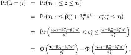
The probability of a given response j_i is

Pr (ji) = Pr(τi-1 < z ≤ τi) = Pr(τi-1 ≤ z ≤ τi) = Fεm (τi) - Fεm (τi-1),

(7)

where F_ε^m is the cumulative distribution function (CDF) of the error term ε^m. When a normal distribution is assumed, the model (7) is called ordered probit.

Note that the Likert scale, as proposed by Likert (1932), has M = 5 levels:

strongly approve,
approve,
undecided,
disapprove,
strongly disapprove.

In the choice context, there are two categories: chosen, or not chosen, so that M = 2. Considering alternative i for individual n, the variable z_in is the difference

z = U - max U in in j jn

(8)

between the utility of alternative i and the largest utility among all alternatives, so that

{ 0 if zin < 0 Iin = 1 if zin ≥ 0

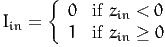(9)

which is (5) with M = 2 and τ₁ = 0.

2 Indirect measurement of latent variables

The indirect measurement of latent variables is usually done by collecting various indicators. A list of statements is provided to the respondent, and she is asked to react to each of them using a Likert scale, as defined above. Although these statements have been designed to capture some pre-determined aspects, it is useful to identify what are the indicators that reveal most of the information about the latent variables.

We consider an example based on data collected in Switzerland in 2009 and 2010 (Atasoy et al., 2011, Atasoy et al., 2013). Various indicators, revealing various attitudes about the environment, about mobility, about residential preferences, and about lifestyle, have been collected, as described in Table 12.

We first perform an exploratory factor analysis on the indicators. For instance, the code in Section B.1 performs this task using the package R (www.r-project.org).

The results are

          Factor1 Factor2 Factor3
Envir01   -0.565
Envir02   -0.407
Envir03    0.414
Mobil11    0.484
Mobil14    0.473
Mobil16    0.462
Mobil17    0.434
Mobil26                    0.408
ResidCh01          0.577
ResidCh04          0.406
ResidCh05          0.635
ResidCh06          0.451
ResidCh07         -0.418
LifSty07           0.430

The first factor is explained by the following indicators:

Envir01: Fuel price should be increased to reduce congestion and air pollution.
Envir02: More public transportation is needed, even if taxes are set to pay the additional costs.
Envir03: Ecology disadvantages minorities and small businesses.
Mobil11: It is difficult to take the public transport when I carry bags or luggage.
Mobil14: When I take the car I know I will be on time.
Mobil16: I do not like changing the mean of transport when I am traveling.
Mobil17: If I use public transportation I have to cancel certain activities I would have done if I had taken the car.

We decide to label the associated latent variable “car lover”. Note the sign of the loading factors, and the associated interpretation of the statements.

In order to write the structural equation (1), we first define some variables from the data file.

age_65_more: the respondent is 65 or older;
moreThanOneCar: the number of cars in the household is strictly greater than 1;
moreThanOneBike: the number of bikes in the household is strictly greater than 1;
individualHouse: the type of house is individual or terraced;
male: the respondent is a male;
haveChildren: the family is a couple or a single with children;
haveGA: the respondent owns a season ticket;
highEducation: the respondent has obtained a degree strictly higher than high school.

We also want to include income. As it is a continuous variable, and strict linearity is not appropriate, we adopt a piecewise linear (or spline) specification. To do so, we define the following variables:

ScaledIncome: income, in 1000 CHF;
ContIncome_0_4000: min(ScaledIncome,4)
ContIncome_4000_6000: max(0,min(ScaledIncome-4,2))
ContIncome_6000_8000: max(0,min(ScaledIncome-6,2))
ContIncome_8000_10000: max(0,min(ScaledIncome-8,2))
ContIncome_10000_more: max(0,ScaledIncome-10)

The structural equation is therefore

* s ∑13 s s x = β0s + k=s1 βkxk + σsε = ¯x + σs ε ,

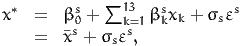(10)

where ε^s is a random variable normally distributed with mean 0 and variance 1:

εs ~ N (0, 1 ),

(11)

and

s s 1∑3 s ¯x = β 0 + β kxk. k=1

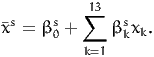(12)

2.1 Indicators as continuous variables

Consider now the measurement equations (3), assuming that the indicators provided by the respondents are continuous, that is that the indicators I_i are used for z in (3). Although this is not formally correct, we assume it first to present corresponding the formulation. We are describing the correct way in Section 2.2.

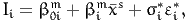
We define the measurement equation for indicator i as

Ii = βm0i + βmi x* + σmi εmi ,

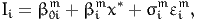(13)

where

εmi ~ N (0, 1).

(14)

Using (10) into (13), we obtain

m m ¯s s m m Ii = β0mi + βim (xs + σsmε ) +s σi εmim = β0i + βi ¯x + β i σs ε + σ i εi .

(15)

The quantity

m s m m β i σs ε + σ i εi

(16)

is normally distributed as

( ) N 0, (σ *i)2 ,

(17)

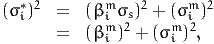
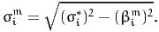
where (σ_i^*)² = (β_i^mσ_s)² + (σ_i^m)². The parameter σ_s is normalized to 1, so that

(σ*)2 = (βm σs)2 + (σm )2 i im 2 m i2 = (β i ) + (σ i ) ,

and

∘ -------------- m * 2 m 2 σi = (σi) - (βi ).

Therefore, we rewrite the measurement equations as

Ii = βm + βm ¯xs + σ*ε*, 0i i i i

(18)

where ε_i^* ~ N(0,1). Not all these parameters can be estimated from data. We need to set the units of the latent variable. It is decided to set it to the first indicator (i = 1), by normalizing β₀₁ = 0 and β₁^m = -1. Note the -1 coefficient, capturing the fact that the first indicator increases when the car loving attitude decreases, as revealed by the factor analysis results, and confirmed by the interpretation.

The implementation of this model in PythonBiogeme is reported in Section B.2.

The statement

loglikelihoodregression(Envir01,MODEL_Envir01,SIGMA_STAR_Envir01)

provides the log likelihood for the linear regression, where Envir01 is the dependent variable I_i, MODEL_Envir01 is the model β_0i^m + β_i^mx^s, CARLOVERS is x^s and SIGMA_STAR_Envir01 is the scale parameter σ_i^*. Note that there are missing data. If the dependent variable is not positive or equal to 6, the value should be ignored and the log likelihood set to 0. This is implemented using the following statement:

Elem({0:0, \
1:loglikelihoodregression(Envir01,MODEL_Envir01,SIGMA_STAR_Envir01)},\
(Envir01 > 0)*(Envir01 < 6))

The dictionary F gathers, for each respondent, the log likelihood of the 7 indicators. The statement

loglike = bioMultSum(F)

calculates the total log likelihood for a given respondent of all 7 indicators together.

The estimation results are reported in Tables 1 and 2, where for each indicator i,

INTER_i is the intercept β_0i^m,
B_i is the coefficient β_i^m,
SIGMA_STAR_i is the scale σ_i^*,

in (18).

Table 1: Estimation results for the linear regression

				Robust
Parameter		Coeff.		Asympt.
number	Description	estimate		std. error		t-stat		p-value

1	INTER_Envir02	2.	01	0.	153	13.	10	0.	00
2	INTER_Envir03	4.	57	0.	158	28.	85	0.	00
3	INTER_Mobil11	5.	14	0.	151	34.	04	0.	00
4	INTER_Mobil14	4.	91	0.	157	31.	21	0.	00
5	INTER_Mobil16	4.	80	0.	158	30.	28	0.	00
6	INTER_Mobil17	4.	50	0.	157	28.	64	0.	00
7	L_Envir02_F1	-0.	496	0.	0578	-8.	59	0.	00
8	L_Envir03_F1	0.	671	0.	0601	11.	16	0.	00
9	L_Mobil11_F1	0.	563	0.	0589	9.	56	0.	00
10	L_Mobil14_F1	0.	705	0.	0596	11.	83	0.	00
11	L_Mobil16_F1	0.	540	0.	0612	8.	82	0.	00
12	L_Mobil17_F1	0.	432	0.	0600	7.	20	0.	00
13	SIGMA_STAR_Envir01	1.	25	0.	0161	77.	34	0.	00
14	SIGMA_STAR_Envir02	1.	12	0.	0149	75.	04	0.	00
15	SIGMA_STAR_Envir03	1.	07	0.	0155	68.	92	0.	00
16	SIGMA_STAR_Mobil11	1.	08	0.	0163	66.	40	0.	00
17	SIGMA_STAR_Mobil14	1.	05	0.	0141	74.	62	0.	00
18	SIGMA_STAR_Mobil16	1.	10	0.	0151	72.	55	0.	00
19	SIGMA_STAR_Mobil17	1.	11	0.	0155	71.	74	0.	00

Table 2: Estimation results for the linear regression (ctd)

				Robust
Parameter		Coeff.		Asympt.
number	Description	estimate		std. error		t-stat		p-value

20	coef_ContIncome_0_4000	0.	103	0.	0633	1.	63	0.	10
21	coef_ContIncome_10000_more	0.	103	0.	0360	2.	86	0.	00
22	coef_ContIncome_4000_6000	-0.	252	0.	108	-2.	33	0.	02
23	coef_ContIncome_6000_8000	0.	300	0.	130	2.	31	0.	02
24	coef_ContIncome_8000_10000	-0.	621	0.	150	-4.	13	0.	00
25	coef_age_65_more	0.	103	0.	0732	1.	41	0.	16
26	coef_haveChildren	-0.	0454	0.	0542	-0.	84	0.	40
27	coef_haveGA	-0.	689	0.	0861	-8.	00	0.	00
28	coef_highEducation	-0.	298	0.	0612	-4.	87	0.	00
29	coef_individualHouse	-0.	110	0.	0540	-2.	04	0.	04
30	coef_intercept	-2.	50	0.	183	-13.	66	0.	00
31	coef_male	0.	0716	0.	0506	1.	41	0.	16
32	coef_moreThanOneBike	-0.	328	0.	0621	-5.	28	0.	00
33	coef_moreThanOneCar	0.	624	0.	0581	10.	74	0.	00

Summary statistics
Number of observations = 1906
Number of excluded observations = 359
Number of estimated parameters = 33
()	=	-20658.648

2.2 Indicators as discrete variables

We now consider the measurement equations (5). As the measurements are using a Likert scale with M = 5 levels, we define 4 parameters τ_i. In order to account for the symmetry of the indicators, we actually define two positive parameters δ₁ and δ₂, and define

τ = -δ - δ 1 1 2 τ2 = -δ1 τ3 = δ1 τ4 = δ1 + δ2

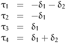
Therefore, the probability of a given response is given by the ordered probit model:

Pr(I = j) = Pr(τ ≤ z ≤ τ ) i i i-1 i = Pr(τi-1 ≤ βm0i + βmix¯s + σ *iε *i ≤ τi) ( ) τi-1-βm0i-βmi ¯xs * τi-βm0i-βmi-¯xs = Pr σ*i < εi ≤ σ*i ( ) ( ) τi-βm0i--βmi ¯xs τi-1-βm0i--βmi ¯xs = Φ σ*i - Φ σ*i ,

(19)

where Φ(⋅) is the CDF of the standardized normal distribution, as illustrated in Figure 1.

PICT

Figure 1: Measurement equation for discrete indicators

The model specification for PythonBiogeme is reported in Section B.3. Equation 19 is coded using the following statements:

Envir01_tau_1 = (tau_1-MODEL_Envir01) / SIGMA_STAR_Envir01
Envir01_tau_2 = (tau_2-MODEL_Envir01) / SIGMA_STAR_Envir01
Envir01_tau_3 = (tau_3-MODEL_Envir01) / SIGMA_STAR_Envir01
Envir01_tau_4 = (tau_4-MODEL_Envir01) / SIGMA_STAR_Envir01
IndEnvir01 = {
    1: bioNormalCdf(Envir01_tau_1),
    2: bioNormalCdf(Envir01_tau_2)-bioNormalCdf(Envir01_tau_1),
    3: bioNormalCdf(Envir01_tau_3)-bioNormalCdf(Envir01_tau_2),
    4: bioNormalCdf(Envir01_tau_4)-bioNormalCdf(Envir01_tau_3),
    5: 1-bioNormalCdf(Envir01_tau_4),
    6: 1.0,
    -1: 1.0,
    -2: 1.0
}

P_Envir01 = Elem(IndEnvir01, Envir01)

Note that the indicators in the data file can take the values -2, -1, 1, 2, 3, 4, 5, and 6. However, the values 6, -1 and 2 are ignored, and associated with a probability of 1, so that they have no influence on the total likelihood function.

Table 3: Estimation results for the ordered probit regression

				Robust
Parameter		Coeff.		Asympt.
number	Description	estimate		std. error		t-stat		p-value

1	B_Envir02_F1	-0.	431	0.	0523	-8.	25	0.	00
2	B_Envir03_F1	0.	566	0.	0531	10.	66	0.	00
3	B_Mobil11_F1	0.	484	0.	0533	9.	09	0.	00
4	B_Mobil14_F1	0.	582	0.	0514	11.	34	0.	00
5	B_Mobil16_F1	0.	463	0.	0543	8.	53	0.	00
6	B_Mobil17_F1	0.	368	0.	0519	7.	10	0.	00
7	INTER_Envir02	0.	349	0.	0261	13.	35	0.	00
8	INTER_Envir03	-0.	309	0.	0270	-11.	42	0.	00
9	INTER_Mobil11	0.	338	0.	0290	11.	66	0.	00
10	INTER_Mobil14	-0.	131	0.	0251	-5.	21	0.	00
11	INTER_Mobil16	0.	128	0.	0276	4.	65	0.	00
12	INTER_Mobil17	0.	146	0.	0260	5.	60	0.	00
13	SIGMA_STAR_Envir02	0.	767	0.	0222	34.	62	0.	00
14	SIGMA_STAR_Envir03	0.	718	0.	0206	34.	89	0.	00
15	SIGMA_STAR_Mobil11	0.	783	0.	0240	32.	63	0.	00
16	SIGMA_STAR_Mobil14	0.	688	0.	0209	32.	98	0.	00
17	SIGMA_STAR_Mobil16	0.	754	0.	0226	33.	42	0.	00
18	SIGMA_STAR_Mobil17	0.	760	0.	0235	32.	32	0.	00

Table 4: Estimation results for the ordered probit regression (ctd)

				Robust
Parameter		Coeff.		Asympt.
number	Description	estimate		std. error		t-stat		p-value

19	coef_ContIncome_0_4000	0.	0903	0.	0528	1.	71	0.	09
20	coef_ContIncome_10000_more	0.	0844	0.	0303	2.	79	0.	01
21	coef_ContIncome_4000_6000	-0.	221	0.	0918	-2.	41	0.	02
22	coef_ContIncome_6000_8000	0.	259	0.	109	2.	37	0.	02
23	coef_ContIncome_8000_10000	-0.	523	0.	128	-4.	10	0.	00
24	coef_age_65_more	0.	0717	0.	0613	1.	17	0.	24
25	coef_haveChildren	-0.	0376	0.	0459	-0.	82	0.	41
26	coef_haveGA	-0.	578	0.	0750	-7.	70	0.	00
27	coef_highEducation	-0.	247	0.	0521	-4.	73	0.	00
28	coef_individualHouse	-0.	0886	0.	0455	-1.	94	0.	05
29	coef_intercept	0.	398	0.	153	2.	61	0.	01
30	coef_male	0.	0664	0.	0433	1.	53	0.	13
31	coef_moreThanOneBike	-0.	277	0.	0538	-5.	15	0.	00
32	coef_moreThanOneCar	0.	533	0.	0516	10.	34	0.	00
33	delta_1	0.	252	0.	00726	34.	70	0.	00
34	delta_2	0.	759	0.	0193	39.	30	0.	00

Summary statistics
Number of observations = 1906
Number of excluded observations = 359
Number of estimated parameters = 34
()	=	-17794.883

3 Choice model

Latent variables can be included in choice models. Consider a model with three alternatives “public transportation” (PT), “car” (CAR) and “slow modes” (SM). The utility functions are of the following form:

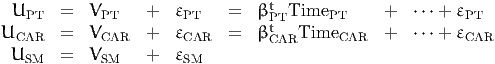t UPT = VPT + εPT = β PtTTimePT + ⋅⋅⋅ + εPT UCAR = VCAR + εCAR = β CARTimeCAR + ⋅⋅⋅ + εCAR USM = VSM + εSM

(20)

The full specification can be found in the specification file in Section B.4. The latent variable that we have considered in the previous sections captures the “car loving” attitude of the individuals. In order to include it in the choice model, we specify that the coefficients of travel time for the public transportation alternative, and for the car alternative, vary with the latent variable. We have

βtPT = β^tPT exp(βCPLTx *),

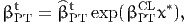(21)

and

βtCAR = ^βtCAR exp (βCCLARx *),

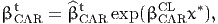(22)

where x^* is defined by (10), so that

t t CL s s β PT = ^β PTexp (βPT (¯x + σsε )),

(23)

and

t ^t CL ¯s s β CAR = βCAR exp (β CAR (x + σsε )).

(24)

Technically, such a choice model can be estimated using the choice observations only, without the indicators. Assuming that ε_PT, ε_CAR and ε_SM are i.i.d. extreme value distributed, we have

s -------------exp(VPT-)------------- Pr (PT |ε ) = exp (V ) + exp (V ) + exp (V ) PT CAR SM

(25)

and

∫ ∞ Pr (PT ) = Pr(PT |ε)ϕ (ε )d ε, ε=-∞

(26)

where ϕ(⋅) is the probability density function of the univariate standardized normal distribution. The choice model is a mixture of logit models. The estimation results are reported in Table 5, where

BETA_TIME_PT_CL refers to βCLPT in (21),
BETA_TIME_PT_REF refers to ^tPT in (21),
BETA_TIME_CAR_CL refers to βCLCAR in (22), and
BETA_TIME_CAR_REF refers to ^tCAR in (22).

Table 5: Estimation results for the mixture of logit models

				Robust
Parameter		Coeff.		Asympt.
number	Description	estimate		std. error		t-stat		p-value

1	ASC_CAR	0.	373	0.	138	2.	70	0.	01
2	ASC_SM	0.	964	0.	263	3.	66	0.	00
3	BETA_COST_HWH	-1.	77	0.	473	-3.	75	0.	00
4	BETA_COST_OTHER	-1.	51	0.	309	-4.	89	0.	00
5	BETA_DIST	-4.	88	0.	655	-7.	46	0.	00
6	BETA_TIME_CAR_CL	-0.	491	0.	0509	-9.	65	0.	00
7	BETA_TIME_CAR_REF	-27.	1	6.	17	-4.	39	0.	00
8	BETA_TIME_PT_CL	-1.	75	0.	0906	-19.	32	0.	00
9	BETA_TIME_PT_REF	-5.	35	2.	85	-1.	88	0.	06
10	BETA_WAITING_TIME	-0.	0517	0.	0175	-2.	96	0.	00
11	coef_ContIncome_0_4000	-0.	102	0.	0907	-1.	12	0.	26
12	coef_ContIncome_10000_more	-0.	101	0.	0354	-2.	86	0.	00
13	coef_ContIncome_4000_6000	0.	0272	0.	121	0.	22	0.	82
14	coef_ContIncome_6000_8000	-0.	125	0.	214	-0.	59	0.	56
15	coef_ContIncome_8000_10000	0.	326	0.	188	1.	73	0.	08
16	coef_age_65_more	0.	199	0.	0858	2.	32	0.	02
17	coef_haveChildren	-0.	0414	0.	0673	-0.	61	0.	54
18	coef_haveGA	1.	33	0.	0869	15.	30	0.	00
19	coef_highEducation	-0.	462	0.	0540	-8.	56	0.	00
20	coef_individualHouse	0.	115	0.	124	0.	92	0.	36
21	coef_male	-0.	133	0.	0567	-2.	35	0.	02
22	coef_moreThanOneBike	0.	152	0.	0977	1.	55	0.	12
23	coef_moreThanOneCar	-0.	598	0.	0669	-8.	94	0.	00

Summary statistics
Number of observations = 1906
Number of excluded observations = 359
Number of estimated parameters = 23
(β₀)	=	-2093.955
()	=	-1078.003
-2[(β₀) - ()]	=	2031.905
ρ²	=	0.485
ρ²	=	0.474

4 Sequential estimation

In order to exploit both the choice data and the psychometric indicator, we now combine the latent variable model with the choice model. The easiest way to estimate a joint model is using sequential estimation. However, such an estimator is not efficient, and a full information estimation is preferable. It is described in Section 5.

For the sequential estimation, we use (10) in (21) and (22), where the values of the coefficients β^s are the result of the estimation presented in Table 3. We have again a mixture of logit models, but with fewer parameters, as the parameters of the structural equation are not re-estimated. The specification file is presented in Section B.5. The estimated parameters of the choice model are presented in Table 6.

It is important to realize that the estimation results in Tables 5 and 6 cannot be compared, as they are not using the same data.

Table 6: Estimation results for the sequential estimation

				Robust
Parameter		Coeff.		Asympt.
number	Description	estimate		std. error		t-stat		p-value

1	ASC_CAR	0.	617	0.	149	4.	14	0.	00
2	ASC_SM	0.	0304	0.	296	0.	10	0.	92
3	BETA_COST_HWH	-1.	79	0.	534	-3.	35	0.	00
4	BETA_COST_OTHER	-1.	20	0.	849	-1.	41	0.	16
5	BETA_DIST	-1.	42	0.	360	-3.	93	0.	00
6	BETA_TIME_CAR_CL	-0.	401	0.	291	-1.	38	0.	17
7	BETA_TIME_CAR_REF	-13.	5	4.	25	-3.	17	0.	00
8	BETA_TIME_PT_CL	0.	662	1.	05	0.	63	0.	53
9	BETA_TIME_PT_REF	-3.	15	2.	02	-1.	56	0.	12
10	BETA_WAITING_TIME	-0.	0519	0.	0307	-1.	69	0.	09

Summary statistics
Number of observations = 1906
Number of excluded observations = 359
Number of estimated parameters = 10
(β₀)	=	-2093.955
()	=	-1174.054
-2[(β₀) - ()]	=	1839.802
ρ²	=	0.439
ρ²	=	0.435

5 Full information estimation

The proper way of estimating the model is to jointly estimate the parameters of the structural equation and the parameters of the choice model, using both the indicators and the choice data.

As the latent variable, and therefore ε^s, is involved in both the measurement equations for the indicators, and the measurement equations of the choice model, the joint likelihood must be first calculated conditional on ε^s:

L (ε) = P (i | ε )∏ Pr(I = j |ε ), n s n n s i in s i

(27)

where i_n is the observed choice of individual n, and j_in is the response of individual n to the psychometric question i. The contribution to the likelihood of this individual is then

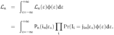∫+ ∞ Ln = Ln (ε)ϕ (ε )d ε ε=-∞ ∫ + ∞ ∏ = Pn (in |εs) Pr(Ii = jin|εs)ϕ (ε)dε. ε=-∞ i

(28)

The specification file is provided in Section B.6, and the estimation results in Tables 7 and 8.

Table 7: Estimation results for the full information estimation

				Robust
Parameter		Coeff.		Asympt.
number	Description	estimate		std. error		t-stat		p-value

1	ASC_CAR	0.	703	0.	118	5.	96	0.	00
2	ASC_SM	0.	261	0.	345	0.	76	0.	45
3	BETA_COST_HWH	-1.	43	0.	341	-4.	19	0.	00
4	BETA_COST_OTHER	-0.	526	0.	161	-3.	27	0.	00
5	BETA_DIST	-1.	41	0.	386	-3.	66	0.	00
6	BETA_TIME_CAR_CL	-0.	956	0.	169	-5.	65	0.	00
7	BETA_TIME_CAR_REF	-9.	50	1.	94	-4.	90	0.	00
8	BETA_TIME_PT_CL	-0.	456	0.	143	-3.	19	0.	00
9	BETA_TIME_PT_REF	-3.	22	0.	838	-3.	84	0.	00
10	BETA_WAITING_TIME	-0.	0205	0.	00962	-2.	13	0.	03
11	B_Envir02_F1	-0.	459	0.	0308	-14.	88	0.	00
12	B_Envir03_F1	0.	484	0.	0316	15.	32	0.	00
13	B_Mobil11_F1	0.	572	0.	0419	13.	65	0.	00
14	B_Mobil14_F1	0.	575	0.	0350	16.	42	0.	00
15	B_Mobil16_F1	0.	525	0.	0425	12.	36	0.	00
16	B_Mobil17_F1	0.	514	0.	0420	12.	25	0.	00
17	INTER_Envir02	0.	460	0.	0308	14.	92	0.	00
18	INTER_Envir03	-0.	367	0.	0289	-12.	69	0.	00
19	INTER_Mobil11	0.	418	0.	0373	11.	22	0.	00
20	INTER_Mobil14	-0.	173	0.	0278	-6.	21	0.	00
21	INTER_Mobil16	0.	148	0.	0336	4.	39	0.	00
22	INTER_Mobil17	0.	140	0.	0329	4.	24	0.	00

Table 8: Estimation results for the full information estimation (ctd.)

				Robust
Parameter		Coeff.		Asympt.
number	Description	estimate		std. error		t-stat		p-value

23	SIGMA_STAR_Envir02	0.	918	0.	0344	26.	63	0.	00
24	SIGMA_STAR_Envir03	0.	857	0.	0352	24.	34	0.	00
25	SIGMA_STAR_Mobil11	0.	895	0.	0409	21.	89	0.	00
26	SIGMA_STAR_Mobil14	0.	759	0.	0333	22.	81	0.	00
27	SIGMA_STAR_Mobil16	0.	873	0.	0397	21.	97	0.	00
28	SIGMA_STAR_Mobil17	0.	876	0.	0392	22.	36	0.	00
29	coef_ContIncome_0_4000	0.	146	0.	0606	2.	41	0.	02
30	coef_ContIncome_10000_more	0.	119	0.	0365	3.	25	0.	00
31	coef_ContIncome_4000_6000	-0.	279	0.	114	-2.	45	0.	01
32	coef_ContIncome_6000_8000	0.	321	0.	137	2.	34	0.	02
33	coef_ContIncome_8000_10000	-0.	666	0.	157	-4.	25	0.	00
34	coef_age_65_more	0.	0403	0.	0748	0.	54	0.	59
35	coef_haveChildren	-0.	0276	0.	0563	-0.	49	0.	62
36	coef_haveGA	-0.	745	0.	0999	-7.	46	0.	00
37	coef_highEducation	-0.	266	0.	0670	-3.	96	0.	00
38	coef_individualHouse	-0.	116	0.	0560	-2.	08	0.	04
39	coef_intercept	0.	373	0.	169	2.	21	0.	03
40	coef_male	0.	0776	0.	0534	1.	45	0.	15
41	coef_moreThanOneBike	-0.	365	0.	0686	-5.	32	0.	00
42	coef_moreThanOneCar	0.	711	0.	0667	10.	66	0.	00
43	delta_1	0.	328	0.	0127	25.	81	0.	00
44	delta_2	0.	989	0.	0358	27.	64	0.	00
45	sigma_s	0.	855	0.	0549	15.	57	0.	00

Summary statistics
Number of observations = 1906
Number of excluded observations = 359
Number of estimated parameters = 45
()	=	-18383.063

6 Serial correlation

The likelihood function (27)–(28) assumes that the error terms involved in the models are independent, that is, ε_i^m in (13), and the errors terms of the utility functions (20). However, because all these models apply to the same individual who made the choice and provided the indicators, these error terms may actually be correlated as they potentially share unobserved variables specific to this individual. This issue, called serial correlation, can be handled by including an agent effect in the model specification. This is an error component appearing in all the models involved, distributed across the individuals.

The specification file is provided in Section B.7, and the estimation results in Tables 9 and 10. In our example, the parameter of the agent affect appears not to be significant, with a p-value of 0.82. Note also that the integral is approximated here using Monte-Carlo simulation.

Table 9: Estimation results for the full information estimation with agent effect

				Robust
Parameter		Coeff.		Asympt.
number	Description	estimate		std. error		t-stat		p-value

1	ASC_CAR	0.	703	0.	118	5.	95	0.	00
2	ASC_SM	0.	261	0.	343	0.	76	0.	45
3	BETA_COST_HWH	-1.	43	0.	340	-4.	21	0.	00
4	BETA_COST_OTHER	-0.	525	0.	161	-3.	27	0.	00
5	BETA_DIST	-1.	41	0.	383	-3.	69	0.	00
6	BETA_TIME_CAR_CL	-0.	953	0.	166	-5.	74	0.	00
7	BETA_TIME_CAR_REF	-9.	50	1.	93	-4.	91	0.	00
8	BETA_TIME_PT_CL	-0.	454	0.	136	-3.	35	0.	00
9	BETA_TIME_PT_REF	-3.	22	0.	838	-3.	85	0.	00
10	BETA_WAITING_TIME	-0.	0204	0.	00962	-2.	12	0.	03
11	B_Envir02_F1	-0.	459	0.	0309	-14.	86	0.	00
12	B_Envir03_F1	0.	484	0.	0316	15.	31	0.	00
13	B_Mobil11_F1	0.	572	0.	0420	13.	62	0.	00
14	B_Mobil14_F1	0.	575	0.	0351	16.	40	0.	00
15	B_Mobil16_F1	0.	525	0.	0426	12.	34	0.	00
16	B_Mobil17_F1	0.	514	0.	0420	12.	23	0.	00
17	INTER_Envir02	0.	460	0.	0308	14.	92	0.	00
18	INTER_Envir03	-0.	367	0.	0289	-12.	69	0.	00
19	INTER_Mobil11	0.	418	0.	0373	11.	22	0.	00
20	INTER_Mobil14	-0.	173	0.	0278	-6.	20	0.	00
21	INTER_Mobil16	0.	147	0.	0337	4.	37	0.	00
22	INTER_Mobil17	0.	140	0.	0329	4.	24	0.	00

Table 10: Estimation results for the full information estimation with agent effect (ctd.)

				Robust
Parameter		Coeff.		Asympt.
number	Description	estimate		std. error		t-stat		p-value

23	SIGMA_STAR_Envir02	0.	918	0.	0345	26.	63	0.	00
24	SIGMA_STAR_Envir03	0.	857	0.	0352	24.	34	0.	00
25	SIGMA_STAR_Mobil11	0.	895	0.	0409	21.	88	0.	00
26	SIGMA_STAR_Mobil14	0.	760	0.	0333	22.	80	0.	00
27	SIGMA_STAR_Mobil16	0.	873	0.	0398	21.	94	0.	00
28	SIGMA_STAR_Mobil17	0.	877	0.	0392	22.	35	0.	00
29	coef_ContIncome_0_4000	0.	147	0.	0606	2.	43	0.	02
30	coef_ContIncome_10000_more	0.	119	0.	0364	3.	26	0.	00
31	coef_ContIncome_4000_6000	-0.	281	0.	114	-2.	47	0.	01
32	coef_ContIncome_6000_8000	0.	322	0.	137	2.	34	0.	02
33	coef_ContIncome_8000_10000	-0.	666	0.	157	-4.	25	0.	00
34	coef_age_65_more	0.	0411	0.	0748	0.	55	0.	58
35	coef_haveChildren	-0.	0253	0.	0566	-0.	45	0.	66
36	coef_haveGA	-0.	743	0.	0999	-7.	44	0.	00
37	coef_highEducation	-0.	267	0.	0669	-3.	99	0.	00
38	coef_individualHouse	-0.	116	0.	0560	-2.	08	0.	04
39	coef_intercept	0.	370	0.	169	2.	19	0.	03
40	coef_male	0.	0773	0.	0534	1.	45	0.	15
41	coef_moreThanOneBike	-0.	366	0.	0688	-5.	32	0.	00
42	coef_moreThanOneCar	0.	710	0.	0668	10.	63	0.	00
43	delta_1	0.	328	0.	0127	25.	80	0.	00
44	delta_2	0.	989	0.	0358	27.	62	0.	00
45	ec_sigma	-0.	0178	0.	0768	-0.	23	0.	82
46	sigma_s	0.	856	0.	0551	15.	55	0.	00

Summary statistics
Number of observations = 1906
Number of excluded observations = 359
Number of estimated parameters = 46
()	=	-18383.598

7 Discussions

We conclude with some comments this short introduction to the estimation of choice models with latent variables.

The initial values of the σ parameters involved in the model specification should be large enough, and in any case certainly not 0. Indeed, if they are too small, the likelihood of some observations may be so small that they are numerically 0. Therefore, calculating the log likelihood is impossible and the estimation will fail even before the first iteration. in this case, PythonBiogeme produces the following message:
Init. log-likelihood: -1.79769e+308 [00:00]
Warning: Error: There is a numerical problem with the initial
log likelihood.  It typically happens when one observation
is associated with a very low probability, so that taking the
log generates a very high number.  Modify the starting values
of the parameters.  You may want to use the SIMULATE feature
of pythonbiogeme to identify the cause of the problem.
The sign of the σ parameters is irrelevant. It is perfectly fine to obtain a negative number.
As discussed above, the estimation of these models involve the calculation of integrals that have no closed form. If there is only one random variable to integrate, it is in general more efficient to use numerical integration, using the Integrate tool of PythonBiogeme. If there are more, Monte-Carlo integration should be preferred. We refer the reader to Bierlaire (2015) for a detailed description of how to do it with PythonBiogeme.
It seems to be common practice to use linear regression on the indicators, assuming that they are continuous variables, as described in Section 2.1. We suggest to avoid that practice, and to prefer an ordered probit formulation as described in Section 2.2, to account for the discrete nature of the indicators. Also, ordered probit should be preferred to ordered logit, as the latter is not based on a symmetric distribution.
It is strongly advised to use the sequential estimation of the model during the model development phase, as the estimation time is significantly reduced. However, once the specification has been finalized, a full information estimation of the parameters should be performed.
The behavioral interpretation of the latent variable is relevant in the context of the indicators that have been collected. When only the choice data are used for the estimation, the interpretation of the latent variable is meaningless as such. It is only relevant in the context of the choice model. It can be seen that the estimates of the parameters using the indicators, presented in Tables 1–2, 3–4 and 7–8 are completely different than the estimates obtained using only the choice data, presented in Table 5. As an example, we illustrate the variation of the latent variable as a function of income in Figure 2, where it is seen that the three estimates involving the indicators capture qualitatively the same pattern, while the one with only the choice data is completely different.

Figure 2: Latent variable as a function of income with the estimated coefficients
We refer the reader to Vij and Walker (2016), who discuss the actual added value (or lack thereof) of using latent variables in the context of a choice model.

A Description of the case study

This case study deals with the estimation of a mode choice behavior model for inhabitants in Switzerland using revealed preference data. The survey was conducted between 2009 and 2010 for CarPostal, the public transport branch of the Swiss Postal Service. The main purpose of this survey is to collect data for analyzing the travel behavior of people in low-density areas, where CarPostal typically serves. A following study proposes new public transport alternatives according to the respondents’ willingness to pay for these potential services in order to increase the market share of public transport.

A.1 Data collection

The survey covers French and German speaking areas of Switzerland. Questionnaires were sent to people living in rural area by mail. The respondents were asked to register all the trips performed during a specified day. The collected information consists of origin, destination, cost, travel time, chosen mode and activity at the destination. Moreover, we collected socio-economic information about the respondents and their households.

1124 completed surveys were collected. For each respondent, cyclic sequences of trips (starting and ending at the same location) are detected and their main transport mode is identified. The resulting data base includes 1906 sequences of trips linked with psychometric indicators and socio-economic attributes of the respondents. It should be noticed that each observation is a sequence of trips that starts and ends at home. A respondent may have several sequences of trips in a day.

A.2 Variables and descriptive statistics

The variables are described in Table 11. The attitudinal statements are described in Table 12. A summary of descriptive statistics for the main variables is given in Table 13.

Given the presence of missing data (coded as -1) an additional table summarizing the three main affected variables (TripPurpose, ReportedDuration, age) after removing the missing cases is presented (see Table 14).



Table 11: Description of variables

Name	Description

ID	Identifier of the respondent who described the trips in the loop.

NbTransf	The total number of transfers performed for all trips of the loop, using public transport (ranging from 1-9).

TimePT	The duration of the loop performed in public transport (in minutes).

WalkingTimePT	The total walking time in a loop performed in public transports (in minutes).

WaitingTimePT	The total waiting time in a loop performed in public transports (in minutes).

TimeCar	The total duration of a loop made using the car (in minutes).

CostPT	Cost for public transports (full cost to perform the loop).

MarginalCostPT	The total cost of a loop performed in public transports, taking into account the ownership of a seasonal ticket by the respondent. If the respondent has a “GA” (full Swiss season ticket), a seasonal ticket for the line or the area, this variable takes value zero. If the respondent has a half-fare travelcard, this variable corresponds to half the cost of the trip by public transport..

CostCarCHF	The total gas cost of a loop performed with the car in CHF.

CostCar	The total gas cost of a loop performed with the car in euros.

TripPurpose	The main purpose of the loop: 1 =Work-related trips; 2 =Work- and leisure-related trips; 3 =Leisure related trips. -1 represents missing values

TypeCommune	The commune type, based on the Swiss Federal Statistical Office 1 =Centers; 2 =Suburban communes; 3 =High-income communes; 4 =Periurban communes; 5 =Touristic communes; 6 =Industrial and tertiary communes; 7 =Rural and commuting communes; 8 =Agricultural and mixed communes; 9 =Agricultural communes

UrbRur	Binary variable, where: 1 =Rural; 2 =Urban.

ClassifCodeLine	Classification of the type of bus lines of the commune: 1 =Center; 2 =Centripetal; 3 =Peripheral; 4 =Feeder.

frequency	Categorical variable for the frequency: 1 =Low frequency, < 12 pairs of trips per day; 2 =Low-middle frequency, 13 - 20 pairs of trips per day; 3 =Middle-high frequency, 21-30 pairs of trips per day; 4 =High frequency, > 30 pairs of trips per day.

NbTrajects	Number of trips in the loop

Region OR CoderegionCAR	Region where the commune of the respondent is situated. These regions are defined by CarPostal as follows: 1 =Vaud; 2 =Valais; 3 =Delemont; 4 =Bern; 5 =Basel, Aargau, Olten; 6 =Zurich; 7 =Eastern Switzerland; 8 =Graubunden.

distance_km	Total distance performed for the loop.


Choice	Choice variable: 0 = public transports (train, bus, tram, etc.); 1 = private modes (car, motorbike, etc.); 2 = soft modes (bike, walk, etc.).

InVehicleTime	Time spent in (on-board) the transport modes only (discarding walking time and waiting time), -1 if missing value.

ReportedDuration	Time spent for the whole loop, as reported by the respondent. -1 represents missing values

LangCode	Language of the commune where the survey was conducted: 1 =French; 2 =German.

age	Age of the respondent (in years) -1 represents missing values.

DestAct	The main activity at destination: 1 is work, 2 is professional trip, 3 is studying, 4 is shopping, 5 is activity at home, 6 is eating/drinking, 7 is personal business, 8 is driving someone, 9 is cultural activity or sport, 10 is going out (with friends, restaurant, cinema, theater), 11 is other and -1 is missing value.

FreqTripHouseh	Frequency of trips related to the household (drive someone, like kids, or shopping), 1 is never, 2 is several times a day, 3 is several times a week, 4 is occasionally, -1 is for missing data and -2 if respondent didn’t answer to any opinion questions.
ModeToSchool	Most often mode used by the respondent to go to school as a kid (> 10), 1 is car (passenger), 2 is train, 3 is public transport, 4 is walking, 5 is biking, 6 is motorbike, 7 is other, 8 is multiple modes, -1 is for missing data and -2 if respondent didn’t answer to any opinion questions.

ResidChild	Main place of residence as a kid (< 18), 1 is city center (large town), 2 is city center (small town), 3 is suburbs, 4 is suburban town, 5 is country side (village), 6 is countryside (isolated), -1 is for missing data and -2 if respondent didn’t answer to any opinion questions.

FreqCarPar	Frequency of the usage of car by the respondent’s parents (or adults in charge) during childhood (< 18), 1 is never, 2 is occasionally, 3 is regularly, 4 is exclusively, -1 is for missing data and -2 if respondent didn’t answer to any opinion questions.

FreqTrainPar	Frequency of the usage of train by the respondent’s parents (or adults in charge) during childhood (< 18), 1 is never, 2 is occasionally, 3 is regularly, 4 is exclusively, -1 is for missing data and -2 if respondent didn’t answer to any opinion questions.

FreqOthPar	Frequency of the usage of tram, bus and other public transport (not train) by the respondent’s parents (or adults in charge) during childhood (< 18), 1 is never, 2 is occasionally, 3 is regularly, 4 is exclusively , -1 is for missing data and -2 if respondent didn’t answer to any opinion questions.

NbHousehold	Number of persons in the household. -1 for missing value.

NbChild	Number of kids (< 15) in the household. -1 for missing value.

NbCar	Number of cars in the household.-1 for missing value.

NbMoto	Number of motorbikes in the household. -1 for missing value.

NbBicy	Number of bikes in the household. -1 for missing value.

NbBicyChild	Number of bikes for kids in the household. -1 for missing value.

NbComp	Number of computers in the household. -1 for missing value.

NbTV	Number of TVs in the household. -1 for missing value.


Internet	Internet connection, 1 is yes, 2 is no. -1 for missing value.

NewsPaperSubs	Newspaper subscription, 1 is yes, 2 is no. -1 for missing value.

NbCellPhones	Number of cell phones in the household (total). -1 for missing value.

NbSmartPhone	Number of smartphones in the household (total). -1 for missing value.

HouseType	House type, 1 is individual house (or terraced house), 2 is apartment (and other types of multi-family residential), 3 is independent room (subletting). -1 for missing value.

OwnHouse	Do you own the place where you are living? 1 is yes, 2 is no. -1 for missing value.

NbRoomsHouse	Number of rooms is your house. -1 for missing value.

YearsInHouse	Number of years spent in the current house. -1 for missing value.

Income	Net monthly income of the household in CHF. 1 is less than 2500, 2 is from 2501 to 4000, 3 is from 4001 to 6000, 4 is from 6001 to 8000, 5 is from 8001 to 10’000 and 6 is more than 10’001. -1 for missing value.

Gender	Gender of the respondent, 1 is man, 2 is woman. -1 for missing value.

BirthYear	Year of birth of the respondent. -1 for missing value.

Mothertongue	Mothertongue. 1 for German or Swiss German, 2 for french, 3 for other, -1 for missing value.

FamilSitu	Familiar situation: 1 is single, 2 is in a couple without children, 3 is in a couple with children, 4 is single with your own children, 5 is in a colocation, 6 is with your parents and 7 is for other situations. -1 for missing values.

OccupStat	What is you occupational status? 1 is for full-time paid professional activity, 2 for partial-time paid professional activity, 3 for searching a job, 4 for occasional employment, 5 for no paid job, 6 for homemaker, 7 for disability leave, 8 for student and 9 for retired. -1 for missing values.

SocioProfCat	To which of the following socio-professional categories do you belong? 1 is for top managers, 2 for intellectual professions, 3 for freelancers, 4 for intermediate professions, 5 for artisans and salespersons, 6 for employees, 7 for workers and 8 for others. -1 for missing values.

Education	Highest education achieved. As mentioned by Wikipedia in English: ”The education system in Switzerland is very diverse, because the constitution of Switzerland delegates the authority for the school system mainly to the cantons. The Swiss constitution sets the foundations, namely that primary school is obligatory for every child and is free in public schools and that the confederation can run or support universities.” (source: http://en.wikipedia.org/wiki/Education_in_Switzerland, accessed April 16, 2013). It is thus difficult to translate the survey that was originally in French and German. The possible answers in the survey are: 1. Unfinished compulsory education: education is compulsory in Switzerland but pupils may finish it at the legal age without succeeding the final exam. 2. Compulsory education with diploma 3. Vocational education: a three or four-year period of training both in a company and following theoretical courses. Ends with a diploma called ”Certificat fédéral de capacité” (i.e., ”professional baccalaureate”) 4. A 3-year generalist school giving access to teaching school, nursing schools, social work school, universities of applied sciences or vocational education (sometime in less than the normal number of years). It does not give access to universities in Switzerland 5. High school: ends with the general baccalaureate exam. The general baccalaureate gives access automatically to universities. 6. Universities of applied sciences, teaching schools, nursing schools, social work schools: ends with a Bachelor and sometimes a Master, mostly focus on vocational training 7. Universities and institutes of technology: ends with an academic Bachelor and in most cases an academic Master 8. PhD thesis

HalfFareST	Is equal to 1 if the respondent has a half-fare travelcard and to 2 if not.

LineRelST	Is equal to 1 if the respondent has a line-related season ticket and 2 if not.

GenAbST	Is equal to 1 if the respondent has a GA (full Swiss season ticket) and 2 if not.

AreaRelST	Is equal to 1 if the respondent has an area-related season ticket and 2 if not.


OtherST	Is equal to 1 if the respondent has a season ticket that was is not in the list and 2 if not.

CarAvail	Represents the availability of a car for the respondent: 1 is always, 2 is sometime, 3 is never. -1 for missing value.



Table 12: Attitude questions. Coding: 1= strongly disagree, 2=disagree, 3=neutral, 4= agree, 5= strongly agree, 6=not applicable, -1= missing value, -2= all answers to attitude questions missing

Name	Description

Envir01	Fuel price should be increased to reduce congestion and air pollution.

Envir02	More public transportation is needed, even if taxes are set to pay the additional costs.

Envir03	Ecology disadvantages minorities and small businesses.

Envir04	People and employment are more important than the environment.

Envir05	I am concerned about global warming.

Envir06	Actions and decision making are needed to limit greenhouse gas emissions.

Mobil01	My trip is a useful transition between home and work.

Mobil02	The trip I must do interferes with other things I would like to do.

Mobil03	I use the time of my trip in a productive way.

Mobil04	Being stuck in traffic bores me.

Mobil05	I reconsider frequently my mode choice.

Mobil06	I use my current mean of transport mode because I have no alternative.

Mobil07	In general, for my activities, I always have a usual mean of transport.

Mobil08	I do not feel comfortable when I travel close to people I do not know.

Mobil09	Taking the bus helps making the city more comfortable and welcoming.

Mobil10	It is difficult to take the public transport when I travel with my children.

Mobil11	It is difficult to take the public transport when I carry bags or luggage.

Mobil12	It is very important to have a beautiful car.


Mobil13	With my car I can go wherever and whenever.

Mobil14	When I take the car I know I will be on time.

Mobil15	I do not like looking for a parking place.

Mobil16	I do not like changing the mean of transport when I am traveling.

Mobil17	If I use public transportation I have to cancel certain activities I would have done if I had taken the car.

Mobil18	CarPostal bus schedules are sometimes difficult to understand.

Mobil19	I know very well which bus/train I have to take to go where I want to.

Mobil20	I know by heart the schedules of the public transports I regularly use.

Mobil21	I can rely on my family to drive me if needed

Mobil22	When I am in a town I don’t know I feel strongly disoriented

Mobil23	I use the internet to check the schedules and the departure times of buses and trains.

Mobil24	I have always used public transports all my life

Mobil25	When I was young my parents took me to all my activities

Mobil26	I know some drivers of the public transports that I use

Mobil27	I think it is important to have the option to talk to the drivers of public transports.

ResidCh01	I like living in a neighborhood where a lot of things happen.

ResidCh02	The accessibility and mobility conditions are important for the choice of housing.

ResidCh03	Most of my friends live in the same region I live in.

ResidCh04	I would like to have access to more services or activities.

ResidCh05	I would like to live in the city center of a big city.


ResidCh06	I would like to live in a town situated in the outskirts of a city.

ResidCh07	I would like to live in the countryside.

LifSty01	I always choose the best products regardless of price.

LifSty02	I always try to find the cheapest alternative.

LifSty03	I can ask for services in my neighborhood without problems.

LifSty04	I would like to spend more time with my family and friends.

LifSty05	Sometimes I would like to take a day off .

LifSty06	I can recognize the social status of other travelers by looking at their cars.

LifSty07	The pleasure of having something beautiful consists in showing it.

LifSty08	For me the car is only a practical way to move.

LifSty09	I would like to spend more time working.

LifSty10	I do not like to be in the same place for too long.

LifSty11	I always plan my activities well in advance

LifSty12	I like to experiment new or different situations

LifSty13	I am not afraid of unknown people

LifSty14	My schedule is rather regular.

Table 13: Descriptive statistics of the main variables (no data excluded)


	nbr. cases	nbr. null	min	max	median	mean	std.dev

age	1906	0	-1	88	47	46.48	18.57

Choice	1906	536	0	2	1	0.78	0.54

TypeCommune	1906	0	1	9	6	5.39	1.99

UrbRur	1906	0	1	2	2	1.51	0.5

ClassifCodeLine	1906	0	1	4	4	3.17	0.97

LangCode	1906	0	1	2	2	1.74	0.44

CoderegionCAR	1906	0	1	8	5	4.58	2.08

CostCarCHF	1906	5	0	67.65	2.98	5.76	8.34

distance_km	1906	1	0	519	18.75	40.38	62.6

TimeCar	1906	28	0	494	26	40.68	47.61

TimePT	1906	7	0	745	85	107.88	86.52

frequency	1906	0	1	4	3	2.84	1.09

ID	1906	0	10350017	96040538	44690042	45878800	23846908

InVehicleTime	1906	66	-128	631	40.5	55.13	57.78

MarginalCostPT	1906	270	0	230	5.6	11.11	16.13

NbTrajects	1906	0	1	9	2	2.04	1.05

NbTransf	1906	644	0	14	2	2.01	2.17

Region	1906	0	1	8	5	4.58	2.08

ReportedDuration	1906	3	-1	855	35	57.73	72.47

TripPurpose	1906	0	-1	3	2	1.94	1.18

WaitingTimePT	1906	693	0	392	5	13.13	22.07

WalkingTimePT	1906	17	0	213	33	39.63	28

Table 14: Descriptive statistics of the main variables affected by missing data (observations with -1 excluded)


	nbr. cases	nbr.null	min	max	median	mean	std.dev

age	1791	0	16	88	48	49.53	14.59

ReportedDuration	1835	3	0	855	37	60	72.92

TripPurpose	1783	0	1	3	3	2.14	0.92

B Complete specification files

B.1 factoranalysis.r

1# Read the data file
2thedata = read.table("../optima.dat",header=TRUE)
3
4# Extract the columns corresponding to the indicators
5indicators = thedata[c("Envir01",
6        "Envir02",
7        "Envir03",
8        "Envir04",
9        "Envir05",
10        "Envir06",
11        "Mobil01",
12        "Mobil02",
13        "Mobil03",
14        "Mobil04",
15        "Mobil05",
16        "Mobil06",
17        "Mobil07",
18        "Mobil08",
19        "Mobil09",
20        "Mobil10",
21        "Mobil11",
22        "Mobil12",
23        "Mobil13",
24        "Mobil14",
25        "Mobil15",
26        "Mobil16",
27        "Mobil17",
28        "Mobil18",
29        "Mobil19",
30        "Mobil20",
31        "Mobil21",
32        "Mobil22",
33        "Mobil23",
34        "Mobil24",
35        "Mobil25",
36        "Mobil26",
37        "Mobil27",
38        "ResidCh01",
39        "ResidCh02",
40        "ResidCh03",
41        "ResidCh04",
42        "ResidCh05",
43        "ResidCh06",
44        "ResidCh07",
45        "LifSty01",
46        "LifSty02",
47        "LifSty03",
48        "LifSty04",
49        "LifSty05",
50        "LifSty06",
51        "LifSty07",
52        "LifSty08",
53        "LifSty09",
54        "LifSty10",
55        "LifSty11",
56        "LifSty12",
57        "LifSty13",
58        "LifSty14")]
59
60# Negative numbers correspond to missing values.
61# For R: NA
62indicators[indicators <= 0] <- NA
63
64# Performs the factor analysis, omitting the missing values,
65# using 3 factors
66fa = factanal(na.omit(indicators),
67              3,
68              rotation="varimax",
69              na.rm=TRUE)
70
71# Print the results in a file
72sink("loadings.txt")
73print(fa,cutoff=0.4, sort=FALSE)

B.2 01oneLatentRegression.py

B.3 02oneLatentOrdered.py

1
2###IMPORT NECESSARY MODULES TO RUN BIOGEME
3from biogeme import *
4from headers import *
5from loglikelihood import *
6from statistics import *
7
8### Variables
9
10# Piecewise linear definition of income
11ScaledIncome = DefineVariable(’ScaledIncome’,\
12                  CalculatedIncome / 1000)
13ContIncome_0_4000 = DefineVariable(’ContIncome_0_4000’,\
14                  min(ScaledIncome,4))
15ContIncome_4000_6000 = DefineVariable(’ContIncome_4000_6000’,\
16                  max(0,min(ScaledIncome-4,2)))
17ContIncome_6000_8000 = DefineVariable(’ContIncome_6000_8000’,\
18                  max(0,min(ScaledIncome-6,2)))
19ContIncome_8000_10000 = DefineVariable(’ContIncome_8000_10000’,\
20                  max(0,min(ScaledIncome-8,2)))
21ContIncome_10000_more = DefineVariable(’ContIncome_10000_more’,\
22                  max(0,ScaledIncome-10))
23
24
25age_65_more = DefineVariable(’age_65_more’,age >= 65)
26moreThanOneCar = DefineVariable(’moreThanOneCar’,NbCar > 1)
27moreThanOneBike = DefineVariable(’moreThanOneBike’,NbBicy > 1)
28individualHouse = DefineVariable(’individualHouse’,\
29                                 HouseType == 1)
30male = DefineVariable(’male’,Gender == 1)
31haveChildren = DefineVariable(’haveChildren’,\
32      ((FamilSitu == 3)+(FamilSitu == 4)) > 0)
33haveGA = DefineVariable(’haveGA’,GenAbST == 1)
34highEducation = DefineVariable(’highEducation’, Education >= 6)
35
36### Coefficients
37coef_intercept = Beta(’coef_intercept’,0.398165,-1000,1000,0 )
38coef_age_65_more = Beta(’coef_age_65_more’,0.0716533,-1000,1000,0 )
39coef_haveGA = Beta(’coef_haveGA’,-0.578005,-1000,1000,0 )
40coef_ContIncome_0_4000 = \
41 Beta(’coef_ContIncome_0_4000’,0.0902761,-1000,1000,0 )
42coef_ContIncome_4000_6000 = \
43 Beta(’coef_ContIncome_4000_6000’,-0.221283,-1000,1000,0 )
44coef_ContIncome_6000_8000 = \
45 Beta(’coef_ContIncome_6000_8000’,0.259466,-1000,1000,0 )
46coef_ContIncome_8000_10000 = \
47 Beta(’coef_ContIncome_8000_10000’,-0.523049,-1000,1000,0 )
48coef_ContIncome_10000_more = \
49 Beta(’coef_ContIncome_10000_more’,0.084351,-1000,1000,0 )
50coef_moreThanOneCar = \
51 Beta(’coef_moreThanOneCar’,0.53301,-1000,1000,0 )
52coef_moreThanOneBike = \
53 Beta(’coef_moreThanOneBike’,-0.277122,-1000,1000,0 )
54coef_individualHouse = \
55 Beta(’coef_individualHouse’,-0.0885649,-1000,1000,0 )
56coef_male = Beta(’coef_male’,0.0663476,-1000,1000,0 )
57coef_haveChildren = Beta(’coef_haveChildren’,-0.0376042,-1000,1000,0 )
58coef_highEducation = Beta(’coef_highEducation’,-0.246687,-1000,1000,0 )
59
60### Latent variable: structural equation
61
62# Note that the expression must be on a single line. In order to
63# write it across several lines, each line must terminate with
64# the \ symbol
65
66CARLOVERS = \
67coef_intercept +\
68coef_age_65_more * age_65_more +\
69coef_ContIncome_0_4000 * ContIncome_0_4000 +\
70coef_ContIncome_4000_6000 * ContIncome_4000_6000 +\
71coef_ContIncome_6000_8000 * ContIncome_6000_8000 +\
72coef_ContIncome_8000_10000 * ContIncome_8000_10000 +\
73coef_ContIncome_10000_more * ContIncome_10000_more +\
74coef_moreThanOneCar * moreThanOneCar +\
75coef_moreThanOneBike * moreThanOneBike +\
76coef_individualHouse * individualHouse +\
77coef_male * male +\
78coef_haveChildren * haveChildren +\
79coef_haveGA * haveGA +\
80coef_highEducation * highEducation
81
82
83### Measurement equations
84
85INTER_Envir01 = Beta(’INTER_Envir01’,0,-10000,10000,1)
86INTER_Envir02 = Beta(’INTER_Envir02’,0.348654,-10000,10000,0 )
87INTER_Envir03 = Beta(’INTER_Envir03’,-0.309023,-10000,10000,0 )
88INTER_Mobil11 = Beta(’INTER_Mobil11’,0.337726,-10000,10000,0 )
89INTER_Mobil14 = Beta(’INTER_Mobil14’,-0.130563,-10000,10000,0 )
90INTER_Mobil16 = Beta(’INTER_Mobil16’,0.128293,-10000,10000,0 )
91INTER_Mobil17 = Beta(’INTER_Mobil17’,0.145876,-10000,10000,0 )
92
93B_Envir01_F1 = Beta(’B_Envir01_F1’,-1,-10000,10000,1)
94B_Envir02_F1 = Beta(’B_Envir02_F1’,-0.431461,-10000,10000,0 )
95B_Envir03_F1 = Beta(’B_Envir03_F1’,0.565903,-10000,10000,0 )
96B_Mobil11_F1 = Beta(’B_Mobil11_F1’,0.483958,-10000,10000,0 )
97B_Mobil14_F1 = Beta(’B_Mobil14_F1’,0.58221,-10000,10000,0 )
98B_Mobil16_F1 = Beta(’B_Mobil16_F1’,0.463139,-10000,10000,0 )
99B_Mobil17_F1 = Beta(’B_Mobil17_F1’,0.368257,-10000,10000,0 )
100
101
102
103MODEL_Envir01 = INTER_Envir01 + B_Envir01_F1 * CARLOVERS
104MODEL_Envir02 = INTER_Envir02 + B_Envir02_F1 * CARLOVERS
105MODEL_Envir03 = INTER_Envir03 + B_Envir03_F1 * CARLOVERS
106MODEL_Mobil11 = INTER_Mobil11 + B_Mobil11_F1 * CARLOVERS
107MODEL_Mobil14 = INTER_Mobil14 + B_Mobil14_F1 * CARLOVERS
108MODEL_Mobil16 = INTER_Mobil16 + B_Mobil16_F1 * CARLOVERS
109MODEL_Mobil17 = INTER_Mobil17 + B_Mobil17_F1 * CARLOVERS
110
111SIGMA_STAR_Envir01 = Beta(’SIGMA_STAR_Envir01’,1,-10000,10000,1)
112SIGMA_STAR_Envir02 = Beta(’SIGMA_STAR_Envir02’,0.767063,-10000,10000,0 )
113SIGMA_STAR_Envir03 = Beta(’SIGMA_STAR_Envir03’,0.717835,-10000,10000,0 )
114SIGMA_STAR_Mobil11 = Beta(’SIGMA_STAR_Mobil11’,0.783358,-10000,10000,0 )
115SIGMA_STAR_Mobil14 = Beta(’SIGMA_STAR_Mobil14’,0.688264,-10000,10000,0 )
116SIGMA_STAR_Mobil16 = Beta(’SIGMA_STAR_Mobil16’,0.754419,-10000,10000,0 )
117SIGMA_STAR_Mobil17 = Beta(’SIGMA_STAR_Mobil17’,0.760104,-10000,10000,0 )
118
119delta_1 = Beta(’delta_1’,0.251983,0,10,0 )
120delta_2 = Beta(’delta_2’,0.759208,0,10,0 )
121tau_1 = -delta_1 - delta_2
122tau_2 = -delta_1
123tau_3 = delta_1
124tau_4 = delta_1 + delta_2
125
126Envir01_tau_1 = (tau_1-MODEL_Envir01) / SIGMA_STAR_Envir01
127Envir01_tau_2 = (tau_2-MODEL_Envir01) / SIGMA_STAR_Envir01
128Envir01_tau_3 = (tau_3-MODEL_Envir01) / SIGMA_STAR_Envir01
129Envir01_tau_4 = (tau_4-MODEL_Envir01) / SIGMA_STAR_Envir01
130IndEnvir01 = {
131    1: bioNormalCdf(Envir01_tau_1),
132    2: bioNormalCdf(Envir01_tau_2)-bioNormalCdf(Envir01_tau_1),
133    3: bioNormalCdf(Envir01_tau_3)-bioNormalCdf(Envir01_tau_2),
134    4: bioNormalCdf(Envir01_tau_4)-bioNormalCdf(Envir01_tau_3),
135    5: 1-bioNormalCdf(Envir01_tau_4),
136    6: 1.0,
137    -1: 1.0,
138    -2: 1.0
139}
140
141P_Envir01 = Elem(IndEnvir01, Envir01)
142
143
144Envir02_tau_1 = (tau_1-MODEL_Envir02) / SIGMA_STAR_Envir02
145Envir02_tau_2 = (tau_2-MODEL_Envir02) / SIGMA_STAR_Envir02
146Envir02_tau_3 = (tau_3-MODEL_Envir02) / SIGMA_STAR_Envir02
147Envir02_tau_4 = (tau_4-MODEL_Envir02) / SIGMA_STAR_Envir02
148IndEnvir02 = {
149    1: bioNormalCdf(Envir02_tau_1),
150    2: bioNormalCdf(Envir02_tau_2)-bioNormalCdf(Envir02_tau_1),
151    3: bioNormalCdf(Envir02_tau_3)-bioNormalCdf(Envir02_tau_2),
152    4: bioNormalCdf(Envir02_tau_4)-bioNormalCdf(Envir02_tau_3),
153    5: 1-bioNormalCdf(Envir02_tau_4),
154    6: 1.0,
155    -1: 1.0,
156    -2: 1.0
157}
158
159P_Envir02 = Elem(IndEnvir02, Envir02)
160
161Envir03_tau_1 = (tau_1-MODEL_Envir03) / SIGMA_STAR_Envir03
162Envir03_tau_2 = (tau_2-MODEL_Envir03) / SIGMA_STAR_Envir03
163Envir03_tau_3 = (tau_3-MODEL_Envir03) / SIGMA_STAR_Envir03
164Envir03_tau_4 = (tau_4-MODEL_Envir03) / SIGMA_STAR_Envir03
165IndEnvir03 = {
166    1: bioNormalCdf(Envir03_tau_1),
167    2: bioNormalCdf(Envir03_tau_2)-bioNormalCdf(Envir03_tau_1),
168    3: bioNormalCdf(Envir03_tau_3)-bioNormalCdf(Envir03_tau_2),
169    4: bioNormalCdf(Envir03_tau_4)-bioNormalCdf(Envir03_tau_3),
170    5: 1-bioNormalCdf(Envir03_tau_4),
171    6: 1.0,
172    -1: 1.0,
173    -2: 1.0
174}
175
176P_Envir03 = Elem(IndEnvir03, Envir03)
177
178Mobil11_tau_1 = (tau_1-MODEL_Mobil11) / SIGMA_STAR_Mobil11
179Mobil11_tau_2 = (tau_2-MODEL_Mobil11) / SIGMA_STAR_Mobil11
180Mobil11_tau_3 = (tau_3-MODEL_Mobil11) / SIGMA_STAR_Mobil11
181Mobil11_tau_4 = (tau_4-MODEL_Mobil11) / SIGMA_STAR_Mobil11
182IndMobil11 = {
183    1: bioNormalCdf(Mobil11_tau_1),
184    2: bioNormalCdf(Mobil11_tau_2)-bioNormalCdf(Mobil11_tau_1),
185    3: bioNormalCdf(Mobil11_tau_3)-bioNormalCdf(Mobil11_tau_2),
186    4: bioNormalCdf(Mobil11_tau_4)-bioNormalCdf(Mobil11_tau_3),
187    5: 1-bioNormalCdf(Mobil11_tau_4),
188    6: 1.0,
189    -1: 1.0,
190    -2: 1.0
191}
192
193P_Mobil11 = Elem(IndMobil11, Mobil11)
194
195Mobil14_tau_1 = (tau_1-MODEL_Mobil14) / SIGMA_STAR_Mobil14
196Mobil14_tau_2 = (tau_2-MODEL_Mobil14) / SIGMA_STAR_Mobil14
197Mobil14_tau_3 = (tau_3-MODEL_Mobil14) / SIGMA_STAR_Mobil14
198Mobil14_tau_4 = (tau_4-MODEL_Mobil14) / SIGMA_STAR_Mobil14
199IndMobil14 = {
200    1: bioNormalCdf(Mobil14_tau_1),
201    2: bioNormalCdf(Mobil14_tau_2)-bioNormalCdf(Mobil14_tau_1),
202    3: bioNormalCdf(Mobil14_tau_3)-bioNormalCdf(Mobil14_tau_2),
203    4: bioNormalCdf(Mobil14_tau_4)-bioNormalCdf(Mobil14_tau_3),
204    5: 1-bioNormalCdf(Mobil14_tau_4),
205    6: 1.0,
206    -1: 1.0,
207    -2: 1.0
208}
209
210P_Mobil14 = Elem(IndMobil14, Mobil14)
211
212Mobil16_tau_1 = (tau_1-MODEL_Mobil16) / SIGMA_STAR_Mobil16
213Mobil16_tau_2 = (tau_2-MODEL_Mobil16) / SIGMA_STAR_Mobil16
214Mobil16_tau_3 = (tau_3-MODEL_Mobil16) / SIGMA_STAR_Mobil16
215Mobil16_tau_4 = (tau_4-MODEL_Mobil16) / SIGMA_STAR_Mobil16
216IndMobil16 = {
217    1: bioNormalCdf(Mobil16_tau_1),
218    2: bioNormalCdf(Mobil16_tau_2)-bioNormalCdf(Mobil16_tau_1),
219    3: bioNormalCdf(Mobil16_tau_3)-bioNormalCdf(Mobil16_tau_2),
220    4: bioNormalCdf(Mobil16_tau_4)-bioNormalCdf(Mobil16_tau_3),
221    5: 1-bioNormalCdf(Mobil16_tau_4),
222    6: 1.0,
223    -1: 1.0,
224    -2: 1.0
225}
226
227P_Mobil16 = Elem(IndMobil16, Mobil16)
228
229Mobil17_tau_1 = (tau_1-MODEL_Mobil17) / SIGMA_STAR_Mobil17
230Mobil17_tau_2 = (tau_2-MODEL_Mobil17) / SIGMA_STAR_Mobil17
231Mobil17_tau_3 = (tau_3-MODEL_Mobil17) / SIGMA_STAR_Mobil17
232Mobil17_tau_4 = (tau_4-MODEL_Mobil17) / SIGMA_STAR_Mobil17
233IndMobil17 = {
234    1: bioNormalCdf(Mobil17_tau_1),
235    2: bioNormalCdf(Mobil17_tau_2)-bioNormalCdf(Mobil17_tau_1),
236    3: bioNormalCdf(Mobil17_tau_3)-bioNormalCdf(Mobil17_tau_2),
237    4: bioNormalCdf(Mobil17_tau_4)-bioNormalCdf(Mobil17_tau_3),
238    5: 1-bioNormalCdf(Mobil17_tau_4),
239    6: 1.0,
240    -1: 1.0,
241    -2: 1.0
242}
243
244P_Mobil17 = Elem(IndMobil17, Mobil17)
245
246
247loglike = log(P_Envir01) + \
248          log(P_Envir02) + \
249          log(P_Envir03) + \
250          log(P_Mobil11) + \
251          log(P_Mobil14) + \
252          log(P_Mobil16) + \
253          log(P_Mobil17)
254
255
256BIOGEME_OBJECT.EXCLUDE =  (Choice   ==  -1 )
257
258
259
260# Defines an iterator on the data
261rowIterator(’obsIter’)
262
263BIOGEME_OBJECT.ESTIMATE = Sum(loglike,’obsIter’)

B.4 03choiceOnly.py

B.5 04latentChoiceSeq.py

B.6 05latentChoiceFull.py

1
2###IMPORT NECESSARY MODULES TO RUN BIOGEME
3from biogeme import *
4from headers import *
5from loglikelihood import *
6from distributions import *
7from statistics import *
8
9### Variables
10
11# Piecewise linear definition of income
12ScaledIncome = DefineVariable(’ScaledIncome’,\
13                  CalculatedIncome / 1000)
14ContIncome_0_4000 = DefineVariable(’ContIncome_0_4000’,\
15                  min(ScaledIncome,4))
16ContIncome_4000_6000 = DefineVariable(’ContIncome_4000_6000’,\
17                  max(0,min(ScaledIncome-4,2)))
18ContIncome_6000_8000 = DefineVariable(’ContIncome_6000_8000’,\
19                  max(0,min(ScaledIncome-6,2)))
20ContIncome_8000_10000 = DefineVariable(’ContIncome_8000_10000’,\
21                  max(0,min(ScaledIncome-8,2)))
22ContIncome_10000_more = DefineVariable(’ContIncome_10000_more’,\
23                  max(0,ScaledIncome-10))
24
25
26age_65_more = DefineVariable(’age_65_more’,age >= 65)
27moreThanOneCar = DefineVariable(’moreThanOneCar’,NbCar > 1)
28moreThanOneBike = DefineVariable(’moreThanOneBike’,NbBicy > 1)
29individualHouse = DefineVariable(’individualHouse’,\
30                                 HouseType == 1)
31male = DefineVariable(’male’,Gender == 1)
32haveChildren = DefineVariable(’haveChildren’,\
33      ((FamilSitu == 3)+(FamilSitu == 4)) > 0)
34haveGA = DefineVariable(’haveGA’,GenAbST == 1)
35highEducation = DefineVariable(’highEducation’, Education >= 6)
36
37### Coefficients
38coef_intercept = Beta(’coef_intercept’,0.0,-1000,1000,0 )
39coef_age_65_more = Beta(’coef_age_65_more’,0.0,-1000,1000,0 )
40coef_haveGA = Beta(’coef_haveGA’,0.0,-1000,1000,0 )
41coef_ContIncome_0_4000 = \
42 Beta(’coef_ContIncome_0_4000’,0.0,-1000,1000,0 )
43coef_ContIncome_4000_6000 = \
44 Beta(’coef_ContIncome_4000_6000’,0.0,-1000,1000,0 )
45coef_ContIncome_6000_8000 = \
46 Beta(’coef_ContIncome_6000_8000’,0.0,-1000,1000,0 )
47coef_ContIncome_8000_10000 = \
48 Beta(’coef_ContIncome_8000_10000’,0.0,-1000,1000,0 )
49coef_ContIncome_10000_more = \
50 Beta(’coef_ContIncome_10000_more’,0.0,-1000,1000,0 )
51coef_moreThanOneCar = \
52 Beta(’coef_moreThanOneCar’,0.0,-1000,1000,0 )
53coef_moreThanOneBike = \
54 Beta(’coef_moreThanOneBike’,0.0,-1000,1000,0 )
55coef_individualHouse = \
56 Beta(’coef_individualHouse’,0.0,-1000,1000,0 )
57coef_male = Beta(’coef_male’,0.0,-1000,1000,0 )
58coef_haveChildren = Beta(’coef_haveChildren’,0.0,-1000,1000,0 )
59coef_highEducation = Beta(’coef_highEducation’,0.0,-1000,1000,0 )
60
61### Latent variable: structural equation
62
63# Note that the expression must be on a single line. In order to
64# write it across several lines, each line must terminate with
65# the \ symbol
66
67omega = RandomVariable(’omega’)
68density = normalpdf(omega)
69sigma_s = Beta(’sigma_s’,1,-1000,1000,0)
70
71CARLOVERS = \
72coef_intercept +\
73coef_age_65_more * age_65_more +\
74coef_ContIncome_0_4000 * ContIncome_0_4000 +\
75coef_ContIncome_4000_6000 * ContIncome_4000_6000 +\
76coef_ContIncome_6000_8000 * ContIncome_6000_8000 +\
77coef_ContIncome_8000_10000 * ContIncome_8000_10000 +\
78coef_ContIncome_10000_more * ContIncome_10000_more +\
79coef_moreThanOneCar * moreThanOneCar +\
80coef_moreThanOneBike * moreThanOneBike +\
81coef_individualHouse * individualHouse +\
82coef_male * male +\
83coef_haveChildren * haveChildren +\
84coef_haveGA * haveGA +\
85coef_highEducation * highEducation +\
86sigma_s * omega
87
88
89### Measurement equations
90
91INTER_Envir01 = Beta(’INTER_Envir01’,0,-10000,10000,1)
92INTER_Envir02 = Beta(’INTER_Envir02’,0.0,-10000,10000,0 )
93INTER_Envir03 = Beta(’INTER_Envir03’,0.0,-10000,10000,0 )
94INTER_Mobil11 = Beta(’INTER_Mobil11’,0.0,-10000,10000,0 )
95INTER_Mobil14 = Beta(’INTER_Mobil14’,0.0,-10000,10000,0 )
96INTER_Mobil16 = Beta(’INTER_Mobil16’,0.0,-10000,10000,0 )
97INTER_Mobil17 = Beta(’INTER_Mobil17’,0.0,-10000,10000,0 )
98
99B_Envir01_F1 = Beta(’B_Envir01_F1’,-1,-10000,10000,1)
100B_Envir02_F1 = Beta(’B_Envir02_F1’,0.0,-10000,10000,0 )
101B_Envir03_F1 = Beta(’B_Envir03_F1’,0.0,-10000,10000,0 )
102B_Mobil11_F1 = Beta(’B_Mobil11_F1’,0.0,-10000,10000,0 )
103B_Mobil14_F1 = Beta(’B_Mobil14_F1’,0.0,-10000,10000,0 )
104B_Mobil16_F1 = Beta(’B_Mobil16_F1’,0.0,-10000,10000,0 )
105B_Mobil17_F1 = Beta(’B_Mobil17_F1’,0.0,-10000,10000,0 )
106
107
108
109MODEL_Envir01 = INTER_Envir01 + B_Envir01_F1 * CARLOVERS
110MODEL_Envir02 = INTER_Envir02 + B_Envir02_F1 * CARLOVERS
111MODEL_Envir03 = INTER_Envir03 + B_Envir03_F1 * CARLOVERS
112MODEL_Mobil11 = INTER_Mobil11 + B_Mobil11_F1 * CARLOVERS
113MODEL_Mobil14 = INTER_Mobil14 + B_Mobil14_F1 * CARLOVERS
114MODEL_Mobil16 = INTER_Mobil16 + B_Mobil16_F1 * CARLOVERS
115MODEL_Mobil17 = INTER_Mobil17 + B_Mobil17_F1 * CARLOVERS
116
117SIGMA_STAR_Envir01 = Beta(’SIGMA_STAR_Envir01’,1,-10000,10000,1)
118SIGMA_STAR_Envir02 = Beta(’SIGMA_STAR_Envir02’,10.0,-10000,10000,0 )
119SIGMA_STAR_Envir03 = Beta(’SIGMA_STAR_Envir03’,10.0,-10000,10000,0 )
120SIGMA_STAR_Mobil11 = Beta(’SIGMA_STAR_Mobil11’,10.0,-10000,10000,0 )
121SIGMA_STAR_Mobil14 = Beta(’SIGMA_STAR_Mobil14’,10.0,-10000,10000,0 )
122SIGMA_STAR_Mobil16 = Beta(’SIGMA_STAR_Mobil16’,10.0,-10000,10000,0 )
123SIGMA_STAR_Mobil17 = Beta(’SIGMA_STAR_Mobil17’,10.0,-10000,10000,0 )
124
125delta_1 = Beta(’delta_1’,1,0,10,0 )
126delta_2 = Beta(’delta_2’,3.0,0,10,0 )
127tau_1 = -delta_1 - delta_2
128tau_2 = -delta_1
129tau_3 = delta_1
130tau_4 = delta_1 + delta_2
131
132Envir01_tau_1 = (tau_1-MODEL_Envir01) / SIGMA_STAR_Envir01
133Envir01_tau_2 = (tau_2-MODEL_Envir01) / SIGMA_STAR_Envir01
134Envir01_tau_3 = (tau_3-MODEL_Envir01) / SIGMA_STAR_Envir01
135Envir01_tau_4 = (tau_4-MODEL_Envir01) / SIGMA_STAR_Envir01
136IndEnvir01 = {
137    1: bioNormalCdf(Envir01_tau_1),
138    2: bioNormalCdf(Envir01_tau_2)-bioNormalCdf(Envir01_tau_1),
139    3: bioNormalCdf(Envir01_tau_3)-bioNormalCdf(Envir01_tau_2),
140    4: bioNormalCdf(Envir01_tau_4)-bioNormalCdf(Envir01_tau_3),
141    5: 1-bioNormalCdf(Envir01_tau_4),
142    6: 1.0,
143    -1: 1.0,
144    -2: 1.0
145}
146
147P_Envir01 = Elem(IndEnvir01, Envir01)
148
149
150Envir02_tau_1 = (tau_1-MODEL_Envir02) / SIGMA_STAR_Envir02
151Envir02_tau_2 = (tau_2-MODEL_Envir02) / SIGMA_STAR_Envir02
152Envir02_tau_3 = (tau_3-MODEL_Envir02) / SIGMA_STAR_Envir02
153Envir02_tau_4 = (tau_4-MODEL_Envir02) / SIGMA_STAR_Envir02
154IndEnvir02 = {
155    1: bioNormalCdf(Envir02_tau_1),
156    2: bioNormalCdf(Envir02_tau_2)-bioNormalCdf(Envir02_tau_1),
157    3: bioNormalCdf(Envir02_tau_3)-bioNormalCdf(Envir02_tau_2),
158    4: bioNormalCdf(Envir02_tau_4)-bioNormalCdf(Envir02_tau_3),
159    5: 1-bioNormalCdf(Envir02_tau_4),
160    6: 1.0,
161    -1: 1.0,
162    -2: 1.0
163}
164
165P_Envir02 = Elem(IndEnvir02, Envir02)
166
167Envir03_tau_1 = (tau_1-MODEL_Envir03) / SIGMA_STAR_Envir03
168Envir03_tau_2 = (tau_2-MODEL_Envir03) / SIGMA_STAR_Envir03
169Envir03_tau_3 = (tau_3-MODEL_Envir03) / SIGMA_STAR_Envir03
170Envir03_tau_4 = (tau_4-MODEL_Envir03) / SIGMA_STAR_Envir03
171IndEnvir03 = {
172    1: bioNormalCdf(Envir03_tau_1),
173    2: bioNormalCdf(Envir03_tau_2)-bioNormalCdf(Envir03_tau_1),
174    3: bioNormalCdf(Envir03_tau_3)-bioNormalCdf(Envir03_tau_2),
175    4: bioNormalCdf(Envir03_tau_4)-bioNormalCdf(Envir03_tau_3),
176    5: 1-bioNormalCdf(Envir03_tau_4),
177    6: 1.0,
178    -1: 1.0,
179    -2: 1.0
180}
181
182P_Envir03 = Elem(IndEnvir03, Envir03)
183
184Mobil11_tau_1 = (tau_1-MODEL_Mobil11) / SIGMA_STAR_Mobil11
185Mobil11_tau_2 = (tau_2-MODEL_Mobil11) / SIGMA_STAR_Mobil11
186Mobil11_tau_3 = (tau_3-MODEL_Mobil11) / SIGMA_STAR_Mobil11
187Mobil11_tau_4 = (tau_4-MODEL_Mobil11) / SIGMA_STAR_Mobil11
188IndMobil11 = {
189    1: bioNormalCdf(Mobil11_tau_1),
190    2: bioNormalCdf(Mobil11_tau_2)-bioNormalCdf(Mobil11_tau_1),
191    3: bioNormalCdf(Mobil11_tau_3)-bioNormalCdf(Mobil11_tau_2),
192    4: bioNormalCdf(Mobil11_tau_4)-bioNormalCdf(Mobil11_tau_3),
193    5: 1-bioNormalCdf(Mobil11_tau_4),
194    6: 1.0,
195    -1: 1.0,
196    -2: 1.0
197}
198
199P_Mobil11 = Elem(IndMobil11, Mobil11)
200
201Mobil14_tau_1 = (tau_1-MODEL_Mobil14) / SIGMA_STAR_Mobil14
202Mobil14_tau_2 = (tau_2-MODEL_Mobil14) / SIGMA_STAR_Mobil14
203Mobil14_tau_3 = (tau_3-MODEL_Mobil14) / SIGMA_STAR_Mobil14
204Mobil14_tau_4 = (tau_4-MODEL_Mobil14) / SIGMA_STAR_Mobil14
205IndMobil14 = {
206    1: bioNormalCdf(Mobil14_tau_1),
207    2: bioNormalCdf(Mobil14_tau_2)-bioNormalCdf(Mobil14_tau_1),
208    3: bioNormalCdf(Mobil14_tau_3)-bioNormalCdf(Mobil14_tau_2),
209    4: bioNormalCdf(Mobil14_tau_4)-bioNormalCdf(Mobil14_tau_3),
210    5: 1-bioNormalCdf(Mobil14_tau_4),
211    6: 1.0,
212    -1: 1.0,
213    -2: 1.0
214}
215
216P_Mobil14 = Elem(IndMobil14, Mobil14)
217
218Mobil16_tau_1 = (tau_1-MODEL_Mobil16) / SIGMA_STAR_Mobil16
219Mobil16_tau_2 = (tau_2-MODEL_Mobil16) / SIGMA_STAR_Mobil16
220Mobil16_tau_3 = (tau_3-MODEL_Mobil16) / SIGMA_STAR_Mobil16
221Mobil16_tau_4 = (tau_4-MODEL_Mobil16) / SIGMA_STAR_Mobil16
222IndMobil16 = {
223    1: bioNormalCdf(Mobil16_tau_1),
224    2: bioNormalCdf(Mobil16_tau_2)-bioNormalCdf(Mobil16_tau_1),
225    3: bioNormalCdf(Mobil16_tau_3)-bioNormalCdf(Mobil16_tau_2),
226    4: bioNormalCdf(Mobil16_tau_4)-bioNormalCdf(Mobil16_tau_3),
227    5: 1-bioNormalCdf(Mobil16_tau_4),
228    6: 1.0,
229    -1: 1.0,
230    -2: 1.0
231}
232
233P_Mobil16 = Elem(IndMobil16, Mobil16)
234
235Mobil17_tau_1 = (tau_1-MODEL_Mobil17) / SIGMA_STAR_Mobil17
236Mobil17_tau_2 = (tau_2-MODEL_Mobil17) / SIGMA_STAR_Mobil17
237Mobil17_tau_3 = (tau_3-MODEL_Mobil17) / SIGMA_STAR_Mobil17
238Mobil17_tau_4 = (tau_4-MODEL_Mobil17) / SIGMA_STAR_Mobil17
239IndMobil17 = {
240    1: bioNormalCdf(Mobil17_tau_1),
241    2: bioNormalCdf(Mobil17_tau_2)-bioNormalCdf(Mobil17_tau_1),
242    3: bioNormalCdf(Mobil17_tau_3)-bioNormalCdf(Mobil17_tau_2),
243    4: bioNormalCdf(Mobil17_tau_4)-bioNormalCdf(Mobil17_tau_3),
244    5: 1-bioNormalCdf(Mobil17_tau_4),
245    6: 1.0,
246    -1: 1.0,
247    -2: 1.0
248}
249
250P_Mobil17 = Elem(IndMobil17, Mobil17)
251
252# Choice model
253
254
255ASC_CAR = Beta(’ASC_CAR’,0,-10000,10000,0)
256ASC_PT = Beta(’ASC_PT’,0,-10000,10000,1)
257ASC_SM = Beta(’ASC_SM’,0,-10000,10000,0)
258BETA_COST_HWH = Beta(’BETA_COST_HWH’,0.0,-10000,10000,0 )
259BETA_COST_OTHER = Beta(’BETA_COST_OTHER’,0.0,-10000,10000,0 )
260BETA_DIST       = Beta(’BETA_DIST’,0.0,-10000,10000,0)
261BETA_TIME_CAR_REF = Beta(’BETA_TIME_CAR_REF’,0.0,-10000,0,0)
262BETA_TIME_CAR_CL = Beta(’BETA_TIME_CAR_CL’,0.0,-10,10,0)
263BETA_TIME_PT_REF = Beta(’BETA_TIME_PT_REF’,0.0,-10000,0,0)
264BETA_TIME_PT_CL = Beta(’BETA_TIME_PT_CL’,0.0,-10,10,0)
265BETA_WAITING_TIME = Beta(’BETA_WAITING_TIME’,0.0,-10000,10000,0 )
266
267TimePT_scaled  = DefineVariable(’TimePT_scaled’, TimePT   /  200 )
268TimeCar_scaled  = DefineVariable(’TimeCar_scaled’, TimeCar   /  200 )
269MarginalCostPT_scaled  = DefineVariable(’MarginalCostPT_scaled’, MarginalCostPT   /  10 )
270CostCarCHF_scaled  = DefineVariable(’CostCarCHF_scaled’, CostCarCHF   /  10 )
271distance_km_scaled  = DefineVariable(’distance_km_scaled’, distance_km   /  5 )
272PurpHWH = DefineVariable(’PurpHWH’, TripPurpose == 1)
273PurpOther = DefineVariable(’PurpOther’, TripPurpose != 1)
274
275
276### DEFINITION OF UTILITY FUNCTIONS:
277
278BETA_TIME_PT = BETA_TIME_PT_REF * exp(BETA_TIME_PT_CL * CARLOVERS)
279
280V0 = ASC_PT + \
281     BETA_TIME_PT * TimePT_scaled + \
282     BETA_WAITING_TIME * WaitingTimePT + \
283     BETA_COST_HWH * MarginalCostPT_scaled * PurpHWH  +\
284     BETA_COST_OTHER * MarginalCostPT_scaled * PurpOther
285
286BETA_TIME_CAR = BETA_TIME_CAR_REF * exp(BETA_TIME_CAR_CL * CARLOVERS)
287
288V1 = ASC_CAR + \
289      BETA_TIME_CAR * TimeCar_scaled + \
290      BETA_COST_HWH * CostCarCHF_scaled * PurpHWH  + \
291      BETA_COST_OTHER * CostCarCHF_scaled * PurpOther
292
293V2 = ASC_SM + BETA_DIST * distance_km_scaled
294
295# Associate utility functions with the numbering of alternatives
296V = {0: V0,
297     1: V1,
298     2: V2}
299
300# Associate the availability conditions with the alternatives.
301# In this example all alternatives are available for each individual.
302av = {0: 1,
303      1: 1,
304      2: 1}
305
306# The choice model is a logit, conditional to the
307# value of the latent variable
308condprob = bioLogit(V,av,Choice)
309
310condlike = P_Envir01 * \
311          P_Envir02 * \
312          P_Envir03 * \
313          P_Mobil11 * \
314          P_Mobil14 * \
315          P_Mobil16 * \
316          P_Mobil17 * \
317          condprob
318
319loglike = log(Integrate(condlike * density,’omega’))
320
321
322BIOGEME_OBJECT.EXCLUDE =  (Choice   ==  -1 )
323
324
325
326# Defines an iterator on the data
327rowIterator(’obsIter’)
328
329BIOGEME_OBJECT.ESTIMATE = Sum(loglike,’obsIter’)

B.7 06serialCorrelation.py

1
2###IMPORT NECESSARY MODULES TO RUN BIOGEME
3from biogeme import *
4from headers import *
5from loglikelihood import *
6from distributions import *
7from statistics import *
8
9### Variables
10
11# Piecewise linear definition of income
12ScaledIncome = DefineVariable(’ScaledIncome’,\
13                  CalculatedIncome / 1000)
14ContIncome_0_4000 = DefineVariable(’ContIncome_0_4000’,\
15                  min(ScaledIncome,4))
16ContIncome_4000_6000 = DefineVariable(’ContIncome_4000_6000’,\
17                  max(0,min(ScaledIncome-4,2)))
18ContIncome_6000_8000 = DefineVariable(’ContIncome_6000_8000’,\
19                  max(0,min(ScaledIncome-6,2)))
20ContIncome_8000_10000 = DefineVariable(’ContIncome_8000_10000’,\
21                  max(0,min(ScaledIncome-8,2)))
22ContIncome_10000_more = DefineVariable(’ContIncome_10000_more’,\
23                  max(0,ScaledIncome-10))
24
25
26age_65_more = DefineVariable(’age_65_more’,age >= 65)
27moreThanOneCar = DefineVariable(’moreThanOneCar’,NbCar > 1)
28moreThanOneBike = DefineVariable(’moreThanOneBike’,NbBicy > 1)
29individualHouse = DefineVariable(’individualHouse’,\
30                                 HouseType == 1)
31male = DefineVariable(’male’,Gender == 1)
32haveChildren = DefineVariable(’haveChildren’,\
33      ((FamilSitu == 3)+(FamilSitu == 4)) > 0)
34haveGA = DefineVariable(’haveGA’,GenAbST == 1)
35highEducation = DefineVariable(’highEducation’, Education >= 6)
36
37### Coefficients
38coef_intercept = Beta(’coef_intercept’,0.0,-1000,1000,0 )
39coef_age_65_more = Beta(’coef_age_65_more’,0.0,-1000,1000,0 )
40coef_haveGA = Beta(’coef_haveGA’,0.0,-1000,1000,0 )
41coef_ContIncome_0_4000 = \
42 Beta(’coef_ContIncome_0_4000’,0.0,-1000,1000,0 )
43coef_ContIncome_4000_6000 = \
44 Beta(’coef_ContIncome_4000_6000’,0.0,-1000,1000,0 )
45coef_ContIncome_6000_8000 = \
46 Beta(’coef_ContIncome_6000_8000’,0.0,-1000,1000,0 )
47coef_ContIncome_8000_10000 = \
48 Beta(’coef_ContIncome_8000_10000’,0.0,-1000,1000,0 )
49coef_ContIncome_10000_more = \
50 Beta(’coef_ContIncome_10000_more’,0.0,-1000,1000,0 )
51coef_moreThanOneCar = \
52 Beta(’coef_moreThanOneCar’,0.0,-1000,1000,0 )
53coef_moreThanOneBike = \
54 Beta(’coef_moreThanOneBike’,0.0,-1000,1000,0 )
55coef_individualHouse = \
56 Beta(’coef_individualHouse’,0.0,-1000,1000,0 )
57coef_male = Beta(’coef_male’,0.0,-1000,1000,0 )
58coef_haveChildren = Beta(’coef_haveChildren’,0.0,-1000,1000,0 )
59coef_highEducation = Beta(’coef_highEducation’,0.0,-1000,1000,0 )
60
61### Latent variable: structural equation
62
63# Note that the expression must be on a single line. In order to
64# write it across several lines, each line must terminate with
65# the \ symbol
66
67omega = bioDraws(’omega’)
68sigma_s = Beta(’sigma_s’,0.855306,-1000,1000,0,’sigma_s’ )
69
70#
71# Deal with serial correlation by including an error
72# component that is individual specific
73#
74errorComponent = bioDraws(’errorComponent’)
75ec_sigma = Beta(’ec_sigma’,1,-1000,1000,0)
76
77CARLOVERS = \
78coef_intercept +\
79coef_age_65_more * age_65_more +\
80coef_ContIncome_0_4000 * ContIncome_0_4000 +\
81coef_ContIncome_4000_6000 * ContIncome_4000_6000 +\
82coef_ContIncome_6000_8000 * ContIncome_6000_8000 +\
83coef_ContIncome_8000_10000 * ContIncome_8000_10000 +\
84coef_ContIncome_10000_more * ContIncome_10000_more +\
85coef_moreThanOneCar * moreThanOneCar +\
86coef_moreThanOneBike * moreThanOneBike +\
87coef_individualHouse * individualHouse +\
88coef_male * male +\
89coef_haveChildren * haveChildren +\
90coef_haveGA * haveGA +\
91coef_highEducation * highEducation +\
92sigma_s * omega+\
93ec_sigma * errorComponent
94
95
96### Measurement equations
97
98INTER_Envir01 = Beta(’INTER_Envir01’,0,-10000,10000,1)
99INTER_Envir02 = Beta(’INTER_Envir02’,0.459881,-10000,10000,0)
100INTER_Envir03 = Beta(’INTER_Envir03’,-0.366801,-10000,10000,0)
101INTER_Mobil11 = Beta(’INTER_Mobil11’,0.418153,-10000,10000,0)
102INTER_Mobil14 = Beta(’INTER_Mobil14’,-0.172704,-10000,10000,0)
103INTER_Mobil16 = Beta(’INTER_Mobil16’,0.147506,-10000,10000,0)
104INTER_Mobil17 = Beta(’INTER_Mobil17’,0.139642,-10000,10000,0)
105
106B_Envir01_F1 = Beta(’B_Envir01_F1’,-1,-10000,10000,1)
107B_Envir02_F1 = Beta(’B_Envir02_F1’,-0.458776,-10000,10000,0)
108B_Envir03_F1 = Beta(’B_Envir03_F1’,0.484092,-10000,10000,0)
109B_Mobil11_F1 = Beta(’B_Mobil11_F1’,0.571806,-10000,10000,0)
110B_Mobil14_F1 = Beta(’B_Mobil14_F1’,0.575274,-10000,10000,0)
111B_Mobil16_F1 = Beta(’B_Mobil16_F1’,0.524587,-10000,10000,0)
112B_Mobil17_F1 = Beta(’B_Mobil17_F1’,0.514145,-10000,10000,0)
113
114
115
116MODEL_Envir01 = INTER_Envir01 + B_Envir01_F1 * CARLOVERS
117MODEL_Envir02 = INTER_Envir02 + B_Envir02_F1 * CARLOVERS
118MODEL_Envir03 = INTER_Envir03 + B_Envir03_F1 * CARLOVERS
119MODEL_Mobil11 = INTER_Mobil11 + B_Mobil11_F1 * CARLOVERS
120MODEL_Mobil14 = INTER_Mobil14 + B_Mobil14_F1 * CARLOVERS
121MODEL_Mobil16 = INTER_Mobil16 + B_Mobil16_F1 * CARLOVERS
122MODEL_Mobil17 = INTER_Mobil17 + B_Mobil17_F1 * CARLOVERS
123
124SIGMA_STAR_Envir01 = Beta(’SIGMA_STAR_Envir01’,1,-10000,10000,1)
125SIGMA_STAR_Envir02 = Beta(’SIGMA_STAR_Envir02’,0.91756,-10000,10000,0)
126SIGMA_STAR_Envir03 = Beta(’SIGMA_STAR_Envir03’,0.856537,-10000,10000,0)
127SIGMA_STAR_Mobil11 = Beta(’SIGMA_STAR_Mobil11’,0.894838,-10000,10000,0)
128SIGMA_STAR_Mobil14 = Beta(’SIGMA_STAR_Mobil14’,0.759384,-10000,10000,0)
129SIGMA_STAR_Mobil16 = Beta(’SIGMA_STAR_Mobil16’,0.873045,-10000,10000,0)
130SIGMA_STAR_Mobil17 = Beta(’SIGMA_STAR_Mobil17’,0.876418,-10000,10000,0)
131
132delta_1 = Beta(’delta_1’,0.327742,0,10,0 )
133delta_2 = Beta(’delta_2’,0.989242,0,10,0 )
134tau_1 = -delta_1 - delta_2
135tau_2 = -delta_1
136tau_3 = delta_1
137tau_4 = delta_1 + delta_2
138
139Envir01_tau_1 = (tau_1-MODEL_Envir01) / SIGMA_STAR_Envir01
140Envir01_tau_2 = (tau_2-MODEL_Envir01) / SIGMA_STAR_Envir01
141Envir01_tau_3 = (tau_3-MODEL_Envir01) / SIGMA_STAR_Envir01
142Envir01_tau_4 = (tau_4-MODEL_Envir01) / SIGMA_STAR_Envir01
143IndEnvir01 = {
144    1: bioNormalCdf(Envir01_tau_1),
145    2: bioNormalCdf(Envir01_tau_2)-bioNormalCdf(Envir01_tau_1),
146    3: bioNormalCdf(Envir01_tau_3)-bioNormalCdf(Envir01_tau_2),
147    4: bioNormalCdf(Envir01_tau_4)-bioNormalCdf(Envir01_tau_3),
148    5: 1-bioNormalCdf(Envir01_tau_4),
149    6: 1.0,
150    -1: 1.0,
151    -2: 1.0
152}
153
154P_Envir01 = Elem(IndEnvir01, Envir01)
155
156
157Envir02_tau_1 = (tau_1-MODEL_Envir02) / SIGMA_STAR_Envir02
158Envir02_tau_2 = (tau_2-MODEL_Envir02) / SIGMA_STAR_Envir02
159Envir02_tau_3 = (tau_3-MODEL_Envir02) / SIGMA_STAR_Envir02
160Envir02_tau_4 = (tau_4-MODEL_Envir02) / SIGMA_STAR_Envir02
161IndEnvir02 = {
162    1: bioNormalCdf(Envir02_tau_1),
163    2: bioNormalCdf(Envir02_tau_2)-bioNormalCdf(Envir02_tau_1),
164    3: bioNormalCdf(Envir02_tau_3)-bioNormalCdf(Envir02_tau_2),
165    4: bioNormalCdf(Envir02_tau_4)-bioNormalCdf(Envir02_tau_3),
166    5: 1-bioNormalCdf(Envir02_tau_4),
167    6: 1.0,
168    -1: 1.0,
169    -2: 1.0
170}
171
172P_Envir02 = Elem(IndEnvir02, Envir02)
173
174Envir03_tau_1 = (tau_1-MODEL_Envir03) / SIGMA_STAR_Envir03
175Envir03_tau_2 = (tau_2-MODEL_Envir03) / SIGMA_STAR_Envir03
176Envir03_tau_3 = (tau_3-MODEL_Envir03) / SIGMA_STAR_Envir03
177Envir03_tau_4 = (tau_4-MODEL_Envir03) / SIGMA_STAR_Envir03
178IndEnvir03 = {
179    1: bioNormalCdf(Envir03_tau_1),
180    2: bioNormalCdf(Envir03_tau_2)-bioNormalCdf(Envir03_tau_1),
181    3: bioNormalCdf(Envir03_tau_3)-bioNormalCdf(Envir03_tau_2),
182    4: bioNormalCdf(Envir03_tau_4)-bioNormalCdf(Envir03_tau_3),
183    5: 1-bioNormalCdf(Envir03_tau_4),
184    6: 1.0,
185    -1: 1.0,
186    -2: 1.0
187}
188
189P_Envir03 = Elem(IndEnvir03, Envir03)
190
191Mobil11_tau_1 = (tau_1-MODEL_Mobil11) / SIGMA_STAR_Mobil11
192Mobil11_tau_2 = (tau_2-MODEL_Mobil11) / SIGMA_STAR_Mobil11
193Mobil11_tau_3 = (tau_3-MODEL_Mobil11) / SIGMA_STAR_Mobil11
194Mobil11_tau_4 = (tau_4-MODEL_Mobil11) / SIGMA_STAR_Mobil11
195IndMobil11 = {
196    1: bioNormalCdf(Mobil11_tau_1),
197    2: bioNormalCdf(Mobil11_tau_2)-bioNormalCdf(Mobil11_tau_1),
198    3: bioNormalCdf(Mobil11_tau_3)-bioNormalCdf(Mobil11_tau_2),
199    4: bioNormalCdf(Mobil11_tau_4)-bioNormalCdf(Mobil11_tau_3),
200    5: 1-bioNormalCdf(Mobil11_tau_4),
201    6: 1.0,
202    -1: 1.0,
203    -2: 1.0
204}
205
206P_Mobil11 = Elem(IndMobil11, Mobil11)
207
208Mobil14_tau_1 = (tau_1-MODEL_Mobil14) / SIGMA_STAR_Mobil14
209Mobil14_tau_2 = (tau_2-MODEL_Mobil14) / SIGMA_STAR_Mobil14
210Mobil14_tau_3 = (tau_3-MODEL_Mobil14) / SIGMA_STAR_Mobil14
211Mobil14_tau_4 = (tau_4-MODEL_Mobil14) / SIGMA_STAR_Mobil14
212IndMobil14 = {
213    1: bioNormalCdf(Mobil14_tau_1),
214    2: bioNormalCdf(Mobil14_tau_2)-bioNormalCdf(Mobil14_tau_1),
215    3: bioNormalCdf(Mobil14_tau_3)-bioNormalCdf(Mobil14_tau_2),
216    4: bioNormalCdf(Mobil14_tau_4)-bioNormalCdf(Mobil14_tau_3),
217    5: 1-bioNormalCdf(Mobil14_tau_4),
218    6: 1.0,
219    -1: 1.0,
220    -2: 1.0
221}
222
223P_Mobil14 = Elem(IndMobil14, Mobil14)
224
225Mobil16_tau_1 = (tau_1-MODEL_Mobil16) / SIGMA_STAR_Mobil16
226Mobil16_tau_2 = (tau_2-MODEL_Mobil16) / SIGMA_STAR_Mobil16
227Mobil16_tau_3 = (tau_3-MODEL_Mobil16) / SIGMA_STAR_Mobil16
228Mobil16_tau_4 = (tau_4-MODEL_Mobil16) / SIGMA_STAR_Mobil16
229IndMobil16 = {
230    1: bioNormalCdf(Mobil16_tau_1),
231    2: bioNormalCdf(Mobil16_tau_2)-bioNormalCdf(Mobil16_tau_1),
232    3: bioNormalCdf(Mobil16_tau_3)-bioNormalCdf(Mobil16_tau_2),
233    4: bioNormalCdf(Mobil16_tau_4)-bioNormalCdf(Mobil16_tau_3),
234    5: 1-bioNormalCdf(Mobil16_tau_4),
235    6: 1.0,
236    -1: 1.0,
237    -2: 1.0
238}
239
240P_Mobil16 = Elem(IndMobil16, Mobil16)
241
242Mobil17_tau_1 = (tau_1-MODEL_Mobil17) / SIGMA_STAR_Mobil17
243Mobil17_tau_2 = (tau_2-MODEL_Mobil17) / SIGMA_STAR_Mobil17
244Mobil17_tau_3 = (tau_3-MODEL_Mobil17) / SIGMA_STAR_Mobil17
245Mobil17_tau_4 = (tau_4-MODEL_Mobil17) / SIGMA_STAR_Mobil17
246IndMobil17 = {
247    1: bioNormalCdf(Mobil17_tau_1),
248    2: bioNormalCdf(Mobil17_tau_2)-bioNormalCdf(Mobil17_tau_1),
249    3: bioNormalCdf(Mobil17_tau_3)-bioNormalCdf(Mobil17_tau_2),
250    4: bioNormalCdf(Mobil17_tau_4)-bioNormalCdf(Mobil17_tau_3),
251    5: 1-bioNormalCdf(Mobil17_tau_4),
252    6: 1.0,
253    -1: 1.0,
254    -2: 1.0
255}
256
257P_Mobil17 = Elem(IndMobil17, Mobil17)
258
259# Choice model
260
261
262ASC_CAR = Beta(’ASC_CAR’,0.703144,-10000,10000,0)
263ASC_PT = Beta(’ASC_PT’,0,-10000,10000,1)
264ASC_SM = Beta(’ASC_SM’,0.261217,-10000,10000,0)
265BETA_COST_HWH = Beta(’BETA_COST_HWH’,-1.43061,-10000,10000,0)
266BETA_COST_OTHER = Beta(’BETA_COST_OTHER’,-0.52555,-10000,10000,0)
267BETA_DIST = Beta(’BETA_DIST’,-1.41373,-10000,10000,0)
268BETA_TIME_CAR_REF = Beta(’BETA_TIME_CAR_REF’,-9.49633,-10000,0,0)
269BETA_TIME_CAR_CL = Beta(’BETA_TIME_CAR_CL’,-0.955607,-10,10,0)
270BETA_TIME_PT_REF = Beta(’BETA_TIME_PT_REF’,-3.22241,-10000,0,0)
271BETA_TIME_PT_CL = Beta(’BETA_TIME_PT_CL’,-0.456234,-10,10,0)
272BETA_WAITING_TIME = Beta(’BETA_WAITING_TIME’,-0.0204706,-10000,10000,0)
273
274TimePT_scaled  = DefineVariable(’TimePT_scaled’, TimePT   /  200 )
275TimeCar_scaled  = DefineVariable(’TimeCar_scaled’, TimeCar   /  200 )
276MarginalCostPT_scaled  = DefineVariable(’MarginalCostPT_scaled’, MarginalCostPT   /  10 )
277CostCarCHF_scaled  = DefineVariable(’CostCarCHF_scaled’, CostCarCHF   /  10 )
278distance_km_scaled  = DefineVariable(’distance_km_scaled’, distance_km   /  5 )
279PurpHWH = DefineVariable(’PurpHWH’, TripPurpose == 1)
280PurpOther = DefineVariable(’PurpOther’, TripPurpose != 1)
281
282
283### DEFINITION OF UTILITY FUNCTIONS:
284
285BETA_TIME_PT = BETA_TIME_PT_REF * exp(BETA_TIME_PT_CL * CARLOVERS)
286
287V0 = ASC_PT + \
288     BETA_TIME_PT * TimePT_scaled + \
289     BETA_WAITING_TIME * WaitingTimePT + \
290     BETA_COST_HWH * MarginalCostPT_scaled * PurpHWH  +\
291     BETA_COST_OTHER * MarginalCostPT_scaled * PurpOther +\
292     ec_sigma * errorComponent
293
294BETA_TIME_CAR = BETA_TIME_CAR_REF * exp(BETA_TIME_CAR_CL * CARLOVERS)
295
296V1 = ASC_CAR + \
297      BETA_TIME_CAR * TimeCar_scaled + \
298      BETA_COST_HWH * CostCarCHF_scaled * PurpHWH  + \
299      BETA_COST_OTHER * CostCarCHF_scaled * PurpOther+\
300      ec_sigma * errorComponent
301
302V2 = ASC_SM + BETA_DIST * distance_km_scaled
303
304# Associate utility functions with the numbering of alternatives
305V = {0: V0,
306     1: V1,
307     2: V2}
308
309# Associate the availability conditions with the alternatives.
310# In this example all alternatives are available for each individual.
311av = {0: 1,
312      1: 1,
313      2: 1}
314
315# The choice model is a logit, conditional to the
316# value of the latent variable
317condprob = bioLogit(V,av,Choice)
318
319condlike = P_Envir01 * \
320          P_Envir02 * \
321          P_Envir03 * \
322          P_Mobil11 * \
323          P_Mobil14 * \
324          P_Mobil16 * \
325          P_Mobil17 * \
326          condprob
327
328loglike = log(MonteCarlo(condlike))
329
330
331BIOGEME_OBJECT.EXCLUDE =  (Choice   ==  -1 )
332
333
334
335# Defines an iterator on the data
336rowIterator(’obsIter’)
337
338BIOGEME_OBJECT.ESTIMATE = Sum(loglike,’obsIter’)
339
340BIOGEME_OBJECT.PARAMETERS[’RandomDistribution’] = "MLHS"
341BIOGEME_OBJECT.DRAWS = { ’omega’: ’NORMAL’,’errorComponent’: ’NORMAL’ }
342BIOGEME_OBJECT.PARAMETERS[’NbrOfDraws’] = "500"

References

Ashok, K., Dillon, W. R. and Yuan, S. (2002). Extending discrete choice models to incorporate attitudinal and other latent variables, Journal of Marketing Research 39(1): 31–46.

Atasoy, B., Glerum, A. and Bierlaire, M. (2011). Mode choice with attitudinal latent class: a swiss case-study, Proceedings of the Second International Choice Modeling Conference, Leeds, UK.

Atasoy, B., Glerum, A. and Bierlaire, M. (2013). Attitudes towards mode choice in switzerland, disP - The Planning Review 49(2): 101–117.

Ben-Akiva, M., Walker, J., Bernardino, A. T., Gopinath, D. A., Morikawa, T. and Polydoropoulou, A. (2002). Integration of choice and latent variable models, Perpetual motion: Travel behaviour research opportunities and application challenges pp. 431–470.

Bierlaire, M. (2015). Monte-carlo integration with pythonbiogeme, Technical Report 150806, Transport and Mobility Laboratory, Ecole Polytechnique Fédérale de Lausanne.

Greene, W. H. and Hensher, D. A. (2003). A latent class model for discrete choice analysis: contrasts with mixed logit, Transportation Research Part B: Methodological 37(8): 681–698.

Likert, R. (1932). A technique for the measurement of attitudes, Archives of psychology 140: 1–55.

Vij, A. and Walker, J. L. (2016). How, when and why integrated choice and latent variable models are latently useful, Transportation Research Part B: Methodological 90: 192–217.

Walker, J. L. (2001). Extended discrete choice models: integrated framework, flexible error structures, and latent variables, PhD thesis, Massachusetts Institute of Technology.