|
|||||||||||||||||||||||||||||||||||||||||||||||||||||||||||||||||||||||||||||||||||||||||||||||||||||||||||||||||||||||||||||||||||||||||
|
|||||||||||||||||||||||||||||||||||||||||||||||||||||||||||||||||||||||||||||||||||||||||||||||||||||||||||||||||||||||||||||||||||||||||


_______________________
at-test against 1
Report TRANSP-OR 170517
Transport and Mobility Laboratory
School of Architecture, Civil and Environmental Engineering
Ecole Polytechnique Fédérale de Lausanne
transp-or.epfl.ch
Series on Biogeme
The package Biogeme (biogeme.epfl.ch) is designed to estimate the parameters of various models using maximum likelihood estimation. But it can also be used to extract indicators from an estimated model. In this document, we describe how to calculate some indicators particularly relevant in the context of discrete choice models: market shares, revenues, elasticities, and willingness to pay. Clearly, the use of the software is not restricted to these indicators, neither to choice models. But these examples illustrate most of the capabilities.
See 01nestedEstimation.py in Section A.1
We consider a case study involving a transportation mode choice model, using revealed preference data collected in Switzerland in 2009 and 2010 (see Atasoy et al., 2013). The model is a nested logit model with 3 alternatives: public transportation, car and slow modes. The utility functions are defined as:
where ASC_CAR, ASC_SM, BETA_TIME_FULLTIME, BETA_TIME_OTHER, BETA_DIST_MALE, BETA_DIST_FEMALE, BETA_DIST_UNREPORTED, BETA_COST, are parameters to be estimated, TimePT_scale, MarginalCostPT_scaled, TimeCar_scale, CostCarCHF_scale, distance_km_scale are attributes and fulltime, notfulltime, male, female, unreportedGender are socio-economic characteristics. The two alternatives “public transportation” and “slow modes” are grouped into a nest. The complete specification is available in the file 01nestedEstimation.py, reported in Section A.1. We refer the reader to Bierlaire (2016) for an introduction to the syntax.
The parameters are estimated using PythonBiogeme. Their values are reported in Table 1. A file named 01nestedEstimation_param.py is also generated. It contains the values of the estimated parameters written in PythonBiogeme syntax, as well as the code necessary to perform a sensitivity analysis. This code provides the variance-covariance matrix of the estimates.
|
|||||||||||||||||||||||||||||||||||||||||||||||||||||||||||||||||||||||||||||||||||||||||||||||||||||||||||||||||||||||||||||||||||||||||
|
|||||||||||||||||||||||||||||||||||||||||||||||||||||||||||||||||||||||||||||||||||||||||||||||||||||||||||||||||||||||||||||||||||||||||
_______________________
at-test against 1
See 02nestedSimulation.py in Section A.2
Once the model has been estimated, it must be used to derive useful indicators. PythonBiogeme provides a simulation feature for this purpose. We start by describing how to calculate market shares using sample enumeration. It is necessary to have a sample of individuals from the population. For each of them, the value of each of the variables involved in the model must be known. Note that it is possible to use the same sample that what used for estimation, but only if it contains revealed preferences data. Indeed, the calculation of indicators require real values for the variables, not values that have been engineered to the sake of estimating parameters, like in stated preferences data. It is the procedure used in this document.
More formally, consider a choice model Pn(i|xn, n) providing the probability
that individual n chooses alternative i within the choice set n, given the
explanatory variables xn. In order to calculate the market shares in the population
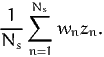
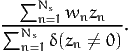
of size N, a sample of Ns individuals is drawn. As it is rarely possible to draw
from the population with equal sampling probability, it is assumed that stratified
sampling has been used, and that each individual n in the sample is associated
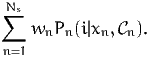
with a weight wn correcting for sampling biases. The weights are normalized such
that
n) providing the probability
that individual n chooses alternative i within the choice set n, given the
explanatory variables xn. In order to calculate the market shares in the population
of size N, a sample of Ns individuals is drawn. As it is rarely possible to draw
from the population with equal sampling probability, it is assumed that stratified
sampling has been used, and that each individual n in the sample is associated
with a weight wn correcting for sampling biases. The weights are normalized such
that
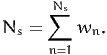 | (1) |
An estimator of the market share of alternative i in the population is
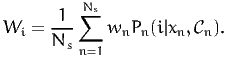 | (2) |
If the alternative i involves a price variable pin, the expected revenue generated by i is
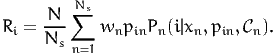 | (3) |
In practice, the size of the population is rarely known, and the above quantity is used only in the context of price optimization. In this case, the factor N∕Ns can be omitted.
To calculate (2) and (3) with PythonBiogeme, a specification file must be prepared. In our example, the file 02nestedSimulation.py, reported in Section A.2, has been produced as follows:
The simulate variable must be a dictionary describing what has to be calculated during the sample enumeration. In this case, we calculate, for each individual in the sample, the choice probability of each alternative. We also calculate the expected revenue generated by each individual for the public transportation companies, using the following statement:
Each entry of this dictionary corresponds to a quantity that will be calculated. The key of the entry is a string, that will be used for the reporting. The value must be a valid formula describing the calculation. In our example, we have defined
calculating the choice probability of each alternative as provided by the nested logit model.
In the output of the estimation (see the file 01nestedEstimation.html), the sum of all weights have been calculated using the statement
The reported result is 0.814484. Therefore, in order to verify (1), we introduce the following statements:
as there are 1906 entries in the data file.
The following statements are included for the calculation of elasticities and will be used later (see Section 3 for more details):
The simulation is performed using the statement
It generates the file 02nestedSimulation.html, that contains the following sections:
 ,
, ), where
  is the
vector of estimated parameters, and
is the
vector of estimated parameters, and  is the variance-covariance matrix
defined by the BIOGEME OBJECT.VARCOVAR statement. The number
of draws is controlled by the parameter NbrOfDrawsForSensitivityAnalysis.
The requested quantity is calculated for each realization, and the
5% and the 95% quantiles of the obtained simulated values
are reported to generate the 90% confidence interval. Note
that the confidence interval is reported only if the statement
is the variance-covariance matrix
defined by the BIOGEME OBJECT.VARCOVAR statement. The number
of draws is controlled by the parameter NbrOfDrawsForSensitivityAnalysis.
The requested quantity is calculated for each realization, and the
5% and the 95% quantiles of the obtained simulated values
are reported to generate the 90% confidence interval. Note
that the confidence interval is reported only if the statement
is present. If you do not need the confidence intervals, simply remove this statement from the .py file.
Therefore, the result of (2) is available in the row “Weighted average”. In this example, the market shares are:
The result of (3) is obtained in the row “Weighted total”. In this case, the expected revenue (generated by the individuals in the sample) is 3018.29 (confidence interval: [2442.87,3826.36]).
Consider now one of the variables involved in the model, for instance xink, the kth variable associated by individual n to alternative i. The objective is to anticipate the impact of a change of the value of this variable on the choice of individual n, and subsequently on the market share of alternative i.
If the variable is continuous, we assume that the relative (infinitesimal) change of the variable is the same for every individual in the population, that is
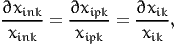 | (14) |
where
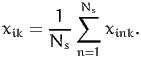 | (15) |
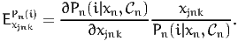
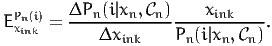
The disaggregate direct point elasticity of the model with respect to the variable xink is defined as
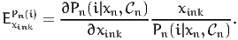 | (16) |
It is called
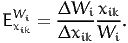
The aggregate direct point elasticity of the model with respect to the average value xik is defined as
 | (17) |
Using (2), we obtain
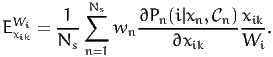 | (18) |
From (14), we obtain
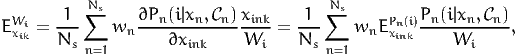 | (19) |
where the second equation is derived from (16). Using (2) again, we obtain
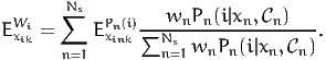 | (20) |
This equation shows that the calculation of aggregate elasticities involves a
weighted sum of disaggregate elasticities. However, the weight is not wn as for the
market share, but a normalized version of wnPn(i|xn,n).
The disaggregate cross point elasticity of the model with respect to the variable xjnk is defined as
 | (21) |
It is called cross elasticity because it measures the sensitivity of the model for alternative i with respect to a modification of the attribute of another alternative.
A similar derivation can be done for arc elasticities. In this case, the relative change of the variable is not infinitesimal anymore. The idea is to analyze a before/after scenario. The variable xink in the before scenario becomes xink + Δxink in the after scenario. As above, we assume that the relative change of the variable is the same for every individual in the population, that is
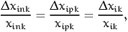 | (22) |
where xik is defined by (15). The disaggregate direct arc elasticity of the model with respect to the variable xink is defined as
 | (23) |
The aggregate direct arc elasticity of the model with respect to the average value xik is defined as
 | (24) |
The two quantities are also related by (20), following the exact same derivation as for the point elasticity.
See 03nestedElasticities.py in Section A.3
The calculation of (16) involves derivatives. For simple models such as logit, the analytical formula of these derivatives can easily be derived. However, their derivation for advanced models can be tedious. It is common to make mistakes in the derivation itself, and even more common to make mistakes in the implementation. Therefore, PythonBiogeme provides an operator that calculates the derivative of a formula. It is illustrated in the file 03nestedElasticities.py, reported in Section A.3. The statements that trigger the calculation of the elasticities are:
The above syntax should be self-explanatory. But there is an important aspect to take into account. In the context of the estimation of the parameters of the model, the variables have been scaled in order to improve the numerical properties of the likelihood function, using statements like
The DefineVariable operator is designed to preprocess the data file, and can be seen as a way to add another column in the data file, defining a new variable. However, the relationship between the new variable and the original one is lost. Therefore, PythonBiogeme is not able to properly calculate the derivatives. In this example, the variable of interest is TimePT, not TimePT_scaled. And their relationship must be explicitly known to correctly calculate the derivatives. Consequently, all statements such as
should be replaced by statements such as
in order to maintain the analytical structure of the formula to be derived.
The aggregate point elasticities can be obtained by aggregating the disaggregate elasticities, using (20). This requires the calculation of the normalization factors
 | (25) |
This has been performed during the previous simulation using the statements
Therefore, we have now included the following statements:
The quantities that must be calculated for each individual in order to derive the aggregate elasticities, correspond to the following entries in the dictionary:
Note that the weights have not been included in the above formula, so that the values of the aggregate elasticities can be found in the row “Weighted total”:
Equivalently, we could have used statements like
and the aggregate value would have been found in the row “Total” instead of “Weighted total’. Note also that we have omitted to report the confidence intervals in this example, by commenting out the statement:
The results are found in the file 03nestedElasticities.html.
See 04nestedElasticities.py in Section A.4
The calculation of (21) is performed in a similar way as the direct elasticities (16), using the following statements:
They calculate the following elasticities:
The corresponding aggregate elasticities are calculated exactly like for the direct case, and their values can be found in the row “Weighted total”.
Note that these values are now positive. Indeed, when the travel time or travel cost of a competing mode increase, the market share increases.
The results are found in the file 04nestedElasticities.html.
See 05nestedElasticities.py in Section A.5
Arc elasticities require a before and after scenarios. In this case, we calculate the sensitivity of the market share of the slow modes alternative when there is a uniform increase of 1 kilometer.
The “before” scenario is represented by the same model as above. The after scenario is modeled using the following statements:
Then, the arc elasticity is calculated as
The aggregate elasticity is calculated as explained above. It is equal here to -1.00708, and the confidence interval is [-1.7212,-0.562574].
The results are found in the file 05nestedElasticities.html.
See 06nestedWTP.py in Section A.6
If the model contains a cost or price variable (like in this example), it is possible to analyze the trade-off between any variable and money. This reflects the willingness of the decision maker to pay for a modification of another variable of the model. A typical example in transportation is the value of time, that is the amount of money a traveler is willing to pay in order to decrease her travel time.
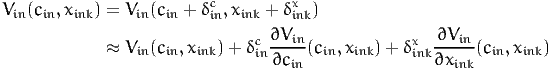
Let cin be the cost of alternative i for individual n. Let xink be the value of another variable of the model. Let Vin(cin,xink) be the value of the utility function. Consider a scenario where the variable of interest takes the value xink + δinkx. We denote by δinc the additional cost that would achieve the same utility, that is
 | (26) |
The willingness to pay to increase the value of xink is defined as the additional cost per unit of x, that is
 | (27) |
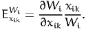
and is obtained by solving Equation (26). If xink and cin appear linearly in the utility function, that is if
 | (28) |
and
 | (29) |
Therefore, (27) is
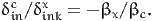 | (30) |
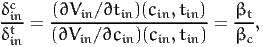
If xink is a continuous variable, and if Vin is differentiable in xink and cin, we can invoke Taylor’s theorem in (26):
 | (31) |
Therefore, the willingness to pay is equal to
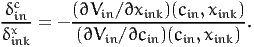 | (32) |
Note that if xink and cin appear linearly in the utility function, (32) is the same as (30). If we consider now a scenario where the variable under interest takes the value xink - δinkx, the same derivation leads to the willingness to pay to decrease the value of xink:
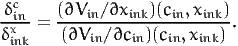 | (33) |
The calculation of the value of time corresponds to such a scenario:
 | (34) |
where the last equation assumes that V is linear in these variables. Note that, in this special case of linear utility functions, the value of time is constant across individuals, and is also independent of δint. This is not true in general.
The calculation of (33) involves the calculation of derivatives. It is done in Pythonbiogeme using the following statements:
The full specification file can be found in Section A.6. The aggregate values are found in the “Weighted average” row of the report file: 3.95822 CHF/hour (confidence interval: [1.98696,7.81565]). Note that this value is abnormally low, which is a sign of a potential poor specification of the model. Note also that, with this specification, the value of time is the same for car and public transportation, as the coefficients of the time and cost variables are generic.
Finally, it is important to look at the distribution of the willingness to pay in the population/sample. The detailed records of the report file allows to do so. It is easy to drag and drop the HTML report file into your favorite spreadsheet software in order to perform additional statistics. In this example, the value of time takes two values, depending on the employment status of the individual:
The results are found in the file 06nestedWTP.html.
PythonBiogeme is a flexible tool that allows to extract useful indicators from complex models. In this document, we have presented how some indicators relevant for discrete choice models can be generated. The HTML format of the report allows to display the report in your favorite browser. It also allows to import the generated values in a spreadsheet for more manipulations.
Available at biogeme.epfl.ch/examples/indicators/python/01nestedEstimation.py
Available at biogeme.epfl.ch/examples/indicators/python/02nestedSimulation.py
Available at biogeme.epfl.ch/examples/indicators/python/03nestedElasticities.py
Available at biogeme.epfl.ch/examples/indicators/python/04nestedElasticities.py
Available at biogeme.epfl.ch/examples/indicators/python/05nestedElasticities.py
Available at biogeme.epfl.ch/examples/indicators/python/06nestedWTP.py
Atasoy, B., Glerum, A. and Bierlaire, M. (2013). Attitudes towards mode choice in switzerland, disP - The Planning Review 49(2): 101–117.
Bierlaire, M. (2016). Pythonbiogeme: a short introduction, Technical Report TRANSP-OR 160706, Transport and Mobility Laboratory, Ecole Polytechnique Fédérale de Lausanne.