The package BisonBiogeme (biogeme.epfl.ch) is designed to estimate the parameters of various models using maximum likelihood estimation. It is particularly designed for discrete choice models. In this document, we present the syntax of the modeling language of BisonBiogeme.

This document is designed to be a reference. We strongly encourage the reader to first consult Bierlaire (2015), where the syntax of a first model is analyzed in details, as well as the many examples provided online. This document has been written using BisonBiogeme 2.4, but should be valid for future versions, as no major release if foreseen.

The model description is written in a file with an extension .mod. The file is organized into sections. Each section starts by a statement like

The sections of this file have to be specified as described below. Note that comments can be included using //. All characters after this command, up to the end of the current line, are ignored.

Note that only relevant sections must be specified. Morevover, the order of the section is irrelevant. However, we suggest to comply to the order as described below.

[ModelDescription]

Type here any text that describes the model. It may contain several lines. Each line must be within double-quotes, like this

[ModelDescription]  
"This is the first line of the model description"  
"This is the second line of the model description"

Note that it will be copied verbatim in the output files. Note that, if it contains special characters which are interpreted by LATEX, such as $ or &, you may need to edit the LATEX output file before processing it.

[Choice]

Provide here the formula to compute the identifier of the chosen alternative from the data file. Typically, a “choice” entry will be available directly in the file, but any formula can be used to compute it. Assume for example that, in your model, you have numbered alternatives 100, 200 and 300. But in the data file, they are numbered 1, 2 and 3. In this case, you must write

      [Choice]  
       100  *  choice  
      

Any expression described in Section [Expressions] is valid here.

[Weight]

Provide here the formula to compute the weight associated with each observation. The weight of an observation will be multiplied to the corresponding term in the log likelihood function. Ideally, the sum of the weights should be equal to the total number of observations, although it is not required. The file reporting the statistics contains a recommendation to adjust the weights in order to comply with this convention.

Important: do not use the weight section in Biosim.

[Beta]

Each line of this section corresponds to a parameter of the utility functions. Five entries must be provided for each parameter:

1. Name: the first character must be a letter (any case) or an underscore (_), followed by a sequence of letters, digits, underscore (_) or dashes (-), and terminated by a white space. Note that case sensitivity is enforced. Therefore varname and Varname would represent two different variables.
2. Default value that will be used as a starting point for the estimation, or used directly for the simulation in BIOSIM.
3. Lower bound on the valid values1 ;
4. Upper bound on the valid values;
5. Status, which is 0 if the parameter must be estimated, or 1 if the parameter has to be maintained at the given default value.

Note that this section is independent of the specific model to be estimated, as it captures the deterministic part of the utility function.

      [Beta]  
      // Name  Value      LowerBound  UpperBound status  
         ASC1  0          -10000      10000      1  
         ASC2  -0.159016  -10000      10000      0  
         ASC3  -0.0869287 -10000      10000      0  
         ASC4  -0.51122   -10000      10000      0  
         ASC5  0.718513   -10000      10000      0  
         ASC6  -1.39177   -10000      10000      0  
         BETA1 0.778982   -10000      10000      0  
         BETA2 0.809772   -10000      10000      0  
      

[Mu]

μ is the homogeneity parameter of the MEV model. Usually, it is constrained to be one. However, BisonBiogeme enables to estimate it if requested (see the Swissmetro example 10nestedBottom.mod for a nested logit model normalized from the bottom, so that μ is estimated). Four entries are specified here:

1. Default value that will be used as a starting point for the estimation (common value: 1.0);
2. Lower bound on the valid values (common value: 1.0e-5);
3. Upper bound on the valid values (common value: 1.0);
4. Status, which is 0 if the parameter must be estimated, or 1 if the parameter has to be maintained at the given value.

[Utilities]

Each row of this section corresponds to an alternative. Four entries are specified:

1. The identifier of the alternative, with a numbering convention consistent with the choice definition;
2. The name of the alternative: the first character must be a letter (any case) or an underscore (_), followed by a sequence of letters, digits, underscore (_) or dashes (-), and terminated by a white space;
3. The availability condition: this must be a direct reference to an entry in the data file, or to an expression defined in the Section [Expressions];
4. The linear-in-parameter utility function is composed of a list of terms, separated by a +. Each term is composed of the name of a parameter and the name of an attribute, separated by a *. The parameter must be listed in Section [Beta], if it is a regular parameter. If it is a random parameter, the syntax is
               nameParam [ nameParam ]  
            

   in the case of the normal distribution, or :

               nameParam { nameParam }  
            

   to get a random parameter that comes from a uniform distribution. For example, in the case of the normal:

               BETA [ SIGMA ]  
            

   Note that the blank after each name parameter is required. Also, parameters BETA and SIGMA have to be listed in Section [Beta]. In the context of an independent random parameter, BETA represents the mean while SIGMA corresponds to the standard deviation. With correlated random parameters, SIGMA technically corresponds to the appropriate term in the Cholesky decomposition matrix that captures the variance-covariance structure among the random parameters. An attribute must be an entry of the data file, or an expression defined in Section [Expressions]. In order to comply with this syntax, the Alternative Specific Constants must appear in a term like ASC * one, where one is defined in the Section [Expressions]. Here is an example:

   [Utilities]  
   // Id Name  Avail  linear-in-parameter expression  
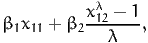
     1   Alt1   av1   ASC1 * one + BETA1 [SIGMA] * x11 + BETA2 * x12  
     2   Alt2   av2   ASC2 * one + BETA1 [SIGMA] * x21 + BETA2 * x22  
     3   Alt3   av3   ASC3 * one + BETA1 [SIGMA] * x31 + BETA2 * x32  
     4   Alt4   av4   ASC4 * one + BETA1 [SIGMA] * x41 + BETA2 * x42  
     5   Alt5   av5   ASC5 * one + BETA1 [SIGMA] * x51 + BETA2 * x52  
     6   Alt6   av6   ASC6 * one + BETA1 [SIGMA] * x61 + BETA2 * x62

   If the utility function does not contain any part which is linear-in-parameters, then the keyword $NONE must be written. For example:

   [Utilities]  
   // Id Name  Avail linear-in-parameter expression  
     1   Alt1   av1  $NONE

[GeneralizedUtilities]

This section enables the user to add nonlinear terms to the utility function. For each alternative, the syntax is simply the identifier of the alternative, followed by the expression. For example, if the utility of alternative 1 is

the syntax is

      [Utilities]  
      1 Alt1 av1 BETA_1 * X11  
 
      [GeneralizedUtilities]  
      1 BETA_2 * (X21 ^ LAMBDA - 1) / LAMBDA  
      

Another example where a nonlinear part is required is when specifying a log normal random coefficient.

[ParameterCovariances]

BisonBiogeme allows normally distributed random parameters to be correlated, and can estimate their covariance. By default, the variance-covariance matrix of the random parameters is supposed to be diagonal, and no covariance is estimated. If some covariances must be estimated, each pair of correlated random coefficients must be identified in this section. Each entry of the section should contain:

1. The name of the first random parameter in the given pair. If it appears in the utility function as BETA [ SIGMA ], its name must be typed BETA_SIGMA.
2. The name of the second random parameter involved in the pair, using the same naming convention.
3. The default value that will be used as a starting point for the estimation;
4. The lower bound on the valid values;
5. The upper bound on the valid values;
6. The status, which is 0 if the parameter must be estimated, or 1 if the parameter has to be maintained at the given value.

If no covariance is to be estimated, you must either entirely remove the section, or specify $NONE as follows:

      [ParameterCovariances]  
      $NONE  
      

[Draws]

Number of draws to be used in Maximum Simulated Likelihood estimation.

[Expressions]

In this section are defined all expressions appearing either in the availability conditions or in the utility functions of the alternatives defined in Section [Utilities]. If the expression is readily available from the data file, it can be omitted in the list. It is good practice to generate new variables from this section especially when one objective is to compute market shares or to evaluate effects of policies with the help of Biosim.

We now summarize the syntax that can be used for generating new variables. Variables which form an expression might be of type float or of type integer. You can use numerical values or the name of a numerical variable. New variables can be created using unary and binary expression operators.

Unary expressions:

1. y = sqrt(x)        // y is square root of x.
2. y = log(x)         // y is natural log of x.
3. y = exp(x)         // y is exponential of x.
4. y = abs(x)         // y is absolute value of x.

binary expression: (Numerical)

1. y = x + z // y is sum of variables x and z
2. y = x - z // y is difference of variables x and z
3. y = x * z // y is product of variables x by z
4. y = x / z // y is division of variable x by z
5. y = x ^ z // y is x to power of z (square would be y = x ^ 2) 
6. y = x % z // y is x modulo z, i.e. rest of x/z 

binary expression: (Logical)

1. y = x == z     // y is 1 if x equals  z, 0 otherwise
2. y = x != z     // y is 1 if x not equal to z, 0 otherwise
3. y = x || z     // y is 1 if x != 0 OR  z != 0, 0 otherwise
4. y = x && z     // y is 1 if x != 0 AND z != 0, 0 otherwise
5. y = x < z      // y is 1 if x < z      (note: also > )
6. y = x <= z     // y is 1 if x <= z     (note: also >= )
7. y = max(x,z)   // y is max of x and z  (note: also min)

Note that an expression is considered to be TRUE if it is non zero, and FALSE if it is zero. For a full description of these expressions and alternative syntaxes, please look at the files patSpecParser.y and patSpecScanner.l in the BIOGEME distribution.

Loops can be defined if several expressions have almost the same syntax. The idea is to replace all occurrences of a string, say xx, by numbers. The numbers are generated within a loop, defined by 3 numbers: the start of the loop (a), the end of the loop (b) and the step (c) with the following syntax:

         $LOOP {xx a b c}  
      

The expression

      $LOOP {xx 1 5 2} my_expression_xx =  
                    other_expression_xx * term_xx_first  
      

is equivalent to

      my_expression_1 = other_expression_1 * term_1_first  
      my_expression_3 = other_expression_3 * term_3_first  
      my_expression_5 = other_expression_5 * term_5_first  
      

Warning: make sure that the string is awkward enough so that it cannot match any other instance by mistake. For example, the loop

      {xp 1 5 2} my_expression_xp = other_expression_xp * term_xp_first  
      

is equivalent to

      my_e1ression_1 = other_e1ression_1 * term_1_first  
      my_e3ression_3 = other_e3ression_3 * term_3_first  
      my_e5ression_5 = other_e5ression_5 * term_5_first  
      

which is probably not the desired effect.

[Group]

Provide here the formula to compute the group ID of the observed individual. Typically, a “group” entry will be available directly from the data file, but any formula can be used to compute it. Any expression described in Section [Expressions] is valid here. A different scale parameter will be estimated for the utility of each group.

[Exclude]

Define an expression (see Section [Expressions]) which identifies entries of the data file to be excluded. If the result of the expression is not zero, the entry will be discarded.

[Model]

Specifies which MEV model is to be used. Valid entries are $BP for Binary Probit, $MNL for Multinomial Logit model, $NL for single level Nested Logit model, $CNL for Cross-Nested Logit model and $NGEV for Network GEV model.

[PanelData]

Used to specify the name of the variable (ex: userID) in the dataset identifying the observations belonging to a given individual and to specify the name of the random parameters that are invariant within the observation of a given individual userID.

[Scale]

A scale parameter is associated with each group. The utility function of each member of a group is multiplied by the associated scale parameter. A typical application is the joined estimation of revealed and stated preferences. It is therefore possible to estimate a logit model combining both data sources, without playing around with dummy nested structures as proposed by Bradley and Daly (1991). Each row of this section corresponds to a group. Five entries are required per row:

1. Group number: the numbering must be consistent with the group definition;
2. Default value that will be used as a starting point for the estimation (1.0 is a good guess);
3. Lower bound on the valid values;
4. Upper bound on the valid values;
5. Status, which is 0 if the parameter must be estimated, or 1 if the parameter has to be maintained at the given value.

Clearly, one of the groups must have a fixed scale parameter.

[SelectionBias]

Identifies the parameters capturing the selection bias, using the estimator proposed by Bierlaire et al. (2008). Each of them has to be listed in Section [Beta]. The section must contain a row per alternative for which a selection bias has to be estimated. Each row contains the number of the alternative and the name of the associated parameter. Note that these parameters play a similar role as the alternative specific constants, and must not be used with logit.

[SelectionBias]  
1 SB_1  
4 SB_4  
6 SB_6

[NLNests]

This section is relevant only if the $NL option has been selected in Section [Model]. If the model to estimate is not a Nested Logit model, the section will simply be ignored. Note that multilevel Nested Logit models must be modeled as Network MEV models. Each row of this section corresponds to a nest. Six entries are required per row:

1. Nest name: the first character must be a letter (any case) or an underscore (_), followed by a sequence of letters, digits, underscore (_) or dashes (-), and terminated by a white space;
2. Default value of the nest parameter μ_m that will be used as a starting point for the estimation (1.0 is a good guess);
3. Lower bound on the valid values. It is usually 1.0, if μ is constrained to be 1.0. Do not forget that, for each nest i, the condition μ_i ≥ μ must be verified to be consistent with discrete choice theory;
4. Upper bound on the valid values;
5. Status, which is 0 if the parameter must be estimated, or 1 if the parameter has to be maintained at the given value.
6. The list of alternatives belonging to the nest, numbered as specified in Section [Utilities]. Make sure that each alternative belongs to exactly one nest, as no automatic verification is implemented in BisonBiogeme.

[CNLNests]

This section is relevant only if the $CNL option has been selected in Section [Model]. If the model to estimate is not a Cross-Nested Logit model, the section will simply be ignored. Note that multilevel Cross-Nested Logit models must be modeled as Network MEV models. Each row of this section corresponds to a nest. Five entries are required per row:

1. Nest name: the first character must be a letter (any case) or an underscore (_), followed by a sequence of letters, digits, underscore (_) or dashes (-), and terminated by a white space;
2. Default value of the nest parameter μ_m that will be used as a starting point for the estimation;
3. Lower bound on the valid values. It is usually 1.0, if μ is constrained to be 1.0. Do not forget that, for each nest i, the condition μ_i ≥ μ must be verified to be consistent with discrete choice theory;
4. Upper bound on the valid values;
5. Status, which is 0 if the parameter must be estimated, or 1 if the parameter has to be maintained at the given value.

[CNLAlpha]

This section is relevant only if the $CNL option has been selected in Section [Model]. If the model to estimate is not a Cross-Nested Logit model, the section will simply be ignored. Each row of this section corresponds to a combination of a nest and an alternative. Six entries are required per row:

1. Alternative name, as defined in Section [Utilities];
2. Nest name: the first character must be a letter (any case) or an underscore (_), followed by a sequence of letters, digits, underscore (_) or dashes (-), and terminated by a white space;
3. Default value of the parameter capturing the level at which an alternative belongs to a nest that will be used as a starting point for the estimation;
4. Lower bound on the valid values (usually 0.0);
5. Upper bound on the valid values (usually 1.0);
6. Status, which is 0 if the parameter must be estimated, or 1 if the parameter has to be maintained at the given value.

[Ratios]

It is sometimes useful to read the ratio of two estimated coefficients. The most typical case is the value-of-time, being the ratio of the time coefficient and the cost coefficient. This feature is only implemented for fixed parameters. Computation of ratio of random parameters is not permitted. Note that it is not straightforward to characterize the distribution of the ratio of two random coefficients. Ben-Akiva et al. (1993) suggest a simple approach that is directly implementable in BIOGEME to handle ratio of random parameters. Each row in this section enables to specify such ratios to be produced in the output file. Three entries are required:

1. The parameter (from Section [Beta]) being the numerator of the ratio;
2. The parameter (from Section [Beta]) being the denominator of the ratio;
3. The name of the ratio, to appear in the output file: the first character must be a letter (any case) or an underscore (_), followed by a sequence of letters, digits, underscore (_) or dashes (-), and terminated by a white space.

[ConstraintNestCoef]

It is possible to constrain nests parameters to be equal. This is achieved by adding to this section expressions like

         NEST_A = NEST_B  
      

where NEST_A and NEST_B are names of nests defined in Section [NLNests], Section [CNLNests] or Section [NetworkGEVNodes]. This section will become obsolete in future releases, as there is now a section for linear constraints on the parameters: (Section [LinearConstraints]).

[NetworkGEVNodes]

This section is relevant only if the $NGEV option has been selected in Section [Model]. If the model to estimate is not a Network GEV model, the section will be simply ignored. Each row of this section corresponds to a node of the Network GEV model. All nodes of the Network GEV model except the root and the alternatives must be listed here, with their associated parameter. Five entries are required per row:

1. Node name: the first character must be a letter (any case) or an underscore (_), followed by a sequence of letters, digits, underscore (_) or dashes (-), and terminated by a white space;
2. Default value of the node parameter μ_j that will be used as a starting point for the estimation;
3. Lower bound on the valid values. It is usually 1.0. Check the condition on the parameters for the model to be consistent with the theory in Bierlaire (2002);
4. Upper bound on the valid values;
5. Status, which is 0 if the parameter must be estimated, or 1 if the parameter has to be maintained at the given value.

[NetworkGEVLinks]

This section is relevant only if the $NGEV option has been selected in Section [Model]. If the model to estimate is not a Network GEV model, the section will be simply ignored. Each row of this section corresponds to a link of the Network GEV model, starting from the a-node to the b-node. The root node is denoted by __ROOT. All other nodes must be either an alternative or a node listed in the section [NetworkGEVNodes]. Note that an alternative cannot be the a-node of any link, and the root node cannot be the b-node of any link. Six entries are required per row:

1. Name of the a-node: it must be either __ROOT or a node listed in the section [NetworkGEVNodes].
2. Name of the b-node: it must be either a node listed in the section [NetworkGEVNodes], or the name of an alternative.
3. Default value of the link parameter that will be used as a starting point for the estimation;
4. Lower bound on the valid values.
5. Upper bound on the valid values;
6. Status, which is 0 if the parameter must be estimated, or 1 if the parameter has to be maintained at the given value.

[LinearConstraints]

In this section, the user can define a list of linear constraints, in one of the following syntaxes:

1. Formula = number,
2. Formula ≤ number,
3. Formula ≥ number.

The syntax is formally defined as follows:

      oneConstraint : equation <= numberParam |  
                  equation = numberParam |  
                  equation >= numberParam  
      equation: eqTerm |  
              - eqTerm |  
              equation + eqTerm  |  
              equation - eqTerm  
      eqTerm: parameter | numberParam * parameter  
      

For example, the constraint

is written

      ASC1 + ASC2 + ASC3 + ASC4 + ASC5 + ASC6 = 0.0  
      

and the constraint

is written

      MU - MUJ <= 0.0  
      

or

      MUJ - MU >= 0.0  
      

[NonLinearEqualityConstraints]

In this section, the user can define a list of nonlinear equality constraints of the form

The section must contain a list of functions h(x). For example, the constraint

is written

      [NonLinearEqualityConstraints]  
      ALPHA_A1 ^ MU_A  + ALPHA_B1 ^ MU_B - 1.0  
      

[NonLinearInequalityConstraints]

BisonBiogeme is not able to handle nonlinear inequality constraints yet. Note that the constraint

is equivalent to

where z is an additional variable (called slack variable).

[DiscreteDistributions]

Provide here the list of random parameters with a discrete distribution, or $NONE if there are none in the model. Each discrete parameter is described using the following syntax:

nameDiscreteParam < listOfDiscreteTerms >

where nameDiscreteParam is the name of the random parameter, and listOfDiscreteTerms is recursively defined as

oneDiscreteTerm |  
listOfDiscreteTerms oneDiscreteTerm

where oneDiscreteTerm is defined as

nameValueParam ( nameProbaParam )

where nameValueParam is the name of the parameter capturing the discrete value of the random parameter, and nameProbaParam is the name of the parameter capturing the associated probability. Both must be defined in Section [Beta]. As an example,

[DiscreteDistributions]  
BETA1 < B1 ( W1 ) B2 ( W2 ) >

defines a random parameter BETA1, which takes the value B1 with probability (or weight) W1, and the value B2 with probability W2. Note that for this to make sense, the constraint W1 + W2 = 1.0 should be imposed (Section [LinearConstraints]). Note also that the parameter BETA1 must not appear in Section [Beta].

[AggregateLast]

This section is relevant when the observation corresponds to a latent choice (see Bierlaire and Frejinger, 2008 and next section). It contains a boolean which, for each row in the sample file, identifies if it is the last observation in an aggregate. Make sure that the value for the last row is nonzero. As all booleans in BisonBiogeme, a numerical value of 0 means “FALSE” and a numerical value different from 0 means “TRUE”. Any expression described in Section [Expressions] is valid here.

[AggregateWeight]

This section is relevant when the observation correspnds to a latent choice. A choice is said to be “latent” when it is not directly observed. This idea has been proposed by Bierlaire and Frejinger (2008) in a route choice context where the actual chosen route was not directly observed. Instead, the respondent reported a sequence of locations that they traversed. In many cases, several routes in the network may have produced the same reported locations.

Each observation consists of an aggregate, a set of actual alternatives that may correspond to the observed situations. If obs is the observed aggregate, than the probability given by the choice model is

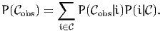(1)

Equation P(obs|i) can be viewed as a measurement equation, and represents the probability to observe obs if i was the actual choice.

In BisonBiogeme, an aggregate observation is represented by a consecutive sequence of elemental observations, associated with the probability P(obs|i). Two additional sections in the model specification file are used for the specification: section [AggregateLast] (see above) and section [AggregateWeight], that associates a weight to elemental observations of an aggregate. It corresponds to the term P(obs|i) in Eq. (1). Any expression described in Section [Expressions] is valid here.

[LaTeX]

This section allows to define a description of each parameter to be used in the LATEX file. For instance, the following section

[LaTeX]  
ASC1   "Constant for alt. 1"  
ASC2   "Constant for alt. 2"  
ASC3   "Constant for alt. 3"  
ASC4   "Constant for alt. 4"  
ASC5   "Constant for alt. 5"  
ASC6   "Constant for alt. 6"  
BETA1  "$\beta_1$"  
BETA2  "$\beta_2$"

will produce the following table:

				Robust
Variable		Coeff.		Asympt.
number	Description	estimate		std. error		t-stat		p-value
1	Constant for alt. 2	-0.	159	0.	106	-1.	49	0.	13
2	Constant for alt. 3	-0.	0869	0.	111	-0.	78	0.	43
3	Constant for alt. 4	-0.	511	0.	172	-2.	97	0.	00
4	Constant for alt. 5	0.	719	0.	158	4.	54	0.	00
5	Constant for alt. 6	-1.	39	0.	195	-7.	12	0.	00
6	β1	0.	779	0.	0301	25.	85	0.	00
7	β2	0.	810	0.	0307	26.	42	0.	00

[Derivatives]

This section is for advanced users only. Use it at your own risk. If you feel that you need it, you may seriously consider using PythonBiogeme instead of BisonBiogeme.

When nonlinear utility functions are used, BisonBiogeme computes automatically the derivatives needed by the maximum likelihood procedure. However, this automatic derivation can significantly slow down the estimation process, as no simplification is performed. This section allows the user to provide BisonBiogeme with the analytical derivatives of the utility function, in order to speed up the estimation process. In some instances, half the estimation time was spared thanks to this feature.

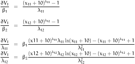
A row must be provided for each combination of nonlinear utilities (defined in the Section Section [GeneralizedUtilities]) and parameters involved in the formula. Each of these rows contains three items:

• the identifier of the alternative,
• the name of the parameter,
• the formula of the derivative.

For instance, assume that the systematic utility of alternative 1 is

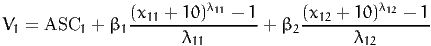
so that

which is coded in BisonBiogeme as follows:

[Utilities]  
// Id Name  Avail  linear-in-parameter expression (beta1*x1 + beta2*x2 + ... )  
  1   Alt1   av1   ASC1 * one  
  .  
  .  
[GeneralizedUtilities]  
1  BETA1 * ((x11 + 10 ) ^ LAMBDA11 - 1) / LAMBDA11 +  
   BETA2 * ((x12 + 10 ) ^ LAMBDA12 - 1) / LAMBDA12  
 
[Derivatives]  
1 BETA1 ((x11 + 10 ) ^ LAMBDA11 - 1) / LAMBDA11  
1 BETA2 ((x12 + 10 ) ^ LAMBDA12 - 1) / LAMBDA12  
1 LAMBDA11  
      BETA1 * ((x11 + 10) ^ LAMBDA11 * LN(x11 + 10) * LAMBDA11  
             - (x11 + 10) ^ LAMBDA11 + 1) / (LAMBDA11 * LAMBDA11 )  
1 LAMBDA12  
      BETA2 * ((x12 + 10) ^ LAMBDA12 * LN(x12 + 10) * LAMBDA12  
             - (x12 + 10) ^ LAMBDA12 + 1) / (LAMBDA12 * LAMBDA12 )

In addition to usual expressions, the formula may contain the following instruction:

$DERIV( formula , param )

which means that you ask BisonBiogeme to perform the derivation of the formula for you. Although it may be useful to simplify the coding of the derivatives, it is mandatory to use it for random parameters.

If BETA [ SIGMA ] is a random parameter, its derivative with respect to BETA is 1, but its derivative with respect to SIGMA cannot be written by the user, and must be coded

$DERIV( BETA [ SIGMA ] , SIGMA )

For instance, assume that the nonlinear utilities are defined as

1 exp( BETA1 [ SIGMA1 ] ) * x11  
2 exp( BETA1 [ SIGMA1 ] ) * x21

The derivatives are coded as follows:

[Derivatives]  
1 BETA1    exp( BETA1 [ SIGMA1 ] ) * x11  
1 SIGMA1   exp( BETA1 [ SIGMA1 ] ) * x11  
              * $DERIV( BETA1 [ SIGMA1 ] , SIGMA1 )  
2 BETA1    exp( BETA1 [ SIGMA1 ] ) * x21  
2 SIGMA1   exp( BETA1 [ SIGMA1 ] ) * x21  
              * $DERIV( BETA1 [ SIGMA1 ] , SIGMA1 )

It is very easy to do an error in coding the analytical derivatives. If there is an error, BisonBiogeme will not be able to estimate the parameters, and will not even be able to detect that there is an error. Therefore, we strongly suggest to set the parameter gevCheckDerivatives to 1 and make sure that the numerical derivatives match sufficiently well the analytical derivatives. Also, estimate the model with few observations and few draws, once with and once without this section. The results should be exactly the same.

[SNP]

This section allows to implement the test proposed by Fosgerau and Bierlaire (2007) (read the paper first if you are not familiar with the test). The section is composed of two things:

1. The name of the random parameter to be tested. If this parameter appears in the utility function as BETA [ SIGMA ], its name in this section must be typed BETA_SIGMA.
2. A list of positive integers associated with a parameter. The integer is the degree of the Legendre polynomial, and the parameter the associated coefficient in the development. Note that the name of the parameter must appear in Section [Beta].

For instance, if parameter BETA [ SIGMA ] is tested using a seminonparametric development defined by

the syntax in BisonBiogeme is

[Beta]  
// Name  Value LowerBound UpperBound  status (0=variable, 1=fixed)  
....  
   BETA  0     -10000     10000       0  
   SIGMA 1     -10000     10000       0  
   SMP1  0     -10000     10000       0  
   SMP3  0     -10000     10000       0  
   SMP4  0     -10000     10000       0  
 
[SNP]  
// Define the coefficients of the series  
// generated by the Legendre polynomials  
BETA_SIGMA  
1 SMP1  
3 SMP3  
4 SMP4

Note that only one random parameter can be transformed at a time.

[OrdinalLogit]

The parameters of ordinal binary logit models can be estimated. However, this feature has not been fully tested, and should be seen as a prototype. Thank you for reporting any bug. The segments of the utility difference space must be numbered in a sequential way, increasing from the leftmost to the rightmost. In this section, each segment must be associated with its lower bound, except the first (because its lower bound is -∞). For instance, if there are 4 segments the following syntax is used:

[Beta]  
....  
tau1 0.3 -1000 1000 1  
tau2 0.4 -1000 1000 0  
tau3 0.5 -1000 1000 0  
 
[OrdinalLogit]  
1 $NONE    //  -infty --> tau1  
2 tau1     //  tau1   --> tau2  
3 tau2     //  tau2   --> tau3  
4 tau3     //  tau3   --> +infty  
 
[LinearConstraints]  
tau1 - tau2 <= 0  
tau2 - tau3 <= 0

Note that the constraints impose that the segments are well-defined. Recall also that the characters // represent a comment in the file and they are not interpreted by BisonBiogeme, as well as all remaining characters on the same line. Therefore, the following syntax for that section is completely equivalent:

[OrdinalLogit]  
1 $NONE  
2 tau1  
3 tau2  
4 tau3

However, we strongly advise to use comments in order to clearly identify the segments.

[SampleEnum]

This section is ignored by BIOGEME. It is used by Biosim and contains the number of simulations to perform in the sample enumeration step.

[ZhengFosgerau]

This section is ignored by BIOGEME. It is used by Biosim and contains instructions to perform the Zheng-Fosgerau specification test and residual analysis. Make sure to read the paper by Fosgerau (2008) before using this section.

There is a line for each test, containing four items:

1. The first item defines the function t introduced by Fosgerau (2008) to reduce the dimensionality of the test. It is typically either the probability of an alternative, or an expression involving coefficients and attributes of the models, as soon as the expression is continuous and not discrete. If it is a probability, the syntax is
   $P { AltName }

   where AltName is the name of the alternative as defined in Section [Utilities]. If it is a general expression, the syntax is

   $E { expr }

   where expr is an expression complying with the syntax of Section [Expressions]. However, it may also contain estimated parameters.

2. The second item is a parameter c used to define the bandwidth for the nonparametric regression performed by the test (see end of Section 2.1 in Fosgerau, 2008). The bandwidth used by Biosim is defined as c∕, where n is the sample size. Most users will use the value c = 1.
3. The third and the fourth item are lower and upper bounds (resp.) Values of t outside of the bounds will not be used in the produced pictures. It is good practice to use wide bounds first, and to adjust them in order to obtain decent pictures. Note that if t is a probability, it does not make sense to have bounds wider and [0 : 1].
4. The last item is the name of the function t, used in the report. Make sure to put the name between double-quotes.

Here is an example of the syntax:

[ZhengFosgerau]  
$P { Alt1 } 1 0 1 "P1"  
$E { x31 } 1 -1000 1000 "x31"

[IIATest]

This section is ignored by BIOGEME. It is used to compute the variables necessary to perform the McFadden omitted variables test on a subset of alternatives:

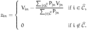(2)

The syntax is illustrated by the following example.

[IIATest]  
// Description of the choice subsets to compute the new  
// variable for McFadden’s IIA test  
// Name list_of_alt  
C123 1 2 3  
C345 3 4 5

Each row corresponds to a new variable. It consists in the name of the variable (it will appear as the column header in the output of Biosim), followed by the list of alternatives to be included in the associated subset.

References