Report TRANSP-OR 150720
Transport and Mobility Laboratory
School of Architecture, Civil and Environmental Engineering
Ecole Polytechnique Fédérale de Lausanne
transp-or.epfl.ch
Series on Biogeme
The package Biogeme (biogeme.epfl.ch) is designed to estimate the parameters of various models using maximum likelihood estimation. It is particularly designed for discrete choice models. In this document, we present step by step how to specify a simple model, estimate its parameters and interpret the output of the software package. We assume that the reader is already familiar with discrete choice models, and has successfully installed BisonBiogeme. This document has been written using BisonBiogeme 2.4, but should be valid for future versions, as no major release if foreseen.
Biogeme assumes that the data file contains in its first line a list of labels corresponding to the available data, and that each subsequent line contains the exact same number of numerical data, each row corresponding to an observation. Delimiters can be tabs or spaces. The tool biopreparedata can be used to transform a file in Comma Separated Version (CSV) into the required format. The tool biocheckdata verifies if the data file complies with the required format.
The data file used for this example is swissmetro.dat. Biogeme is available in two versions. BisonBiogeme is designed to estimate the parameters of a list of predetermined discrete choice models such as logit, binary probit, nested logit, cross-nested logit, multivariate extreme value models, discrete and continuous mixtures of multivariate extreme value models, models with nonlinear utility functions, models designed for panel data, and heteroscedastic models. It is based on a formal and simple language for model specification. PythonBiogeme is designed for general purpose parametric models. The specification of the model and of the likelihood function is based on an extension of the python programming language. A series of discrete choice models are precoded for an easy use.
In this document, we describe the model specification for BisonBiogeme.
The model is a logit model with 3 alternatives: train, Swissmetro and car. The utility functions are defined as:
where TRAIN_TT_SCALED, TRAIN_COST_SCALED, SM_TT_SCALED, SM_COST_SCALED, CAR_TT_SCALED, CAR_CO_SCALED are variables, and ASC_TRAIN, ASC_SM, ASC_CAR, B_TIME, B_COST are parameters to be estimated. Note that it is not possible to identify all alternative specific constants ASC_TRAIN, ASC_SM, ASC_CAR from data. Consequently, ASC_SM is normalized to 0.
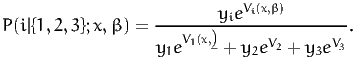
The availability of an alternative i is determined by the variable yi, i=1,...3, which is equal to 1 if the alternative is available, 0 otherwise. The probability of choosing an available alternative i is given by the logit model:
|
| (1) |
Given a data set of N observations, the log likelihood of the sample is
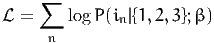 | (2) |
where in is the alternative actually chosen by individual n.
The model specification file must have an extension .mod. The file 01logit.mod is reported in Section A.1. We describe here its content.
The model specification is organized into sections. The order in which the sections appear in the file is not important for BisonBiogeme. Each section starts with the name of the section within square brackets, such as [ModelDescription] or [Choice]. The file can contain also comments, designed to document the specification. Comments are included using the characters //. All characters after this command, up to the end of the current line, are ignored by BisonBiogeme. In our example, the file starts with comments describing the name of the file, its author and the date when it was created. A short description of its content is also provided.
These comments are completely ignored by BisonBiogeme. However, it is recommended to use many comments to describe the model specification, for future reference, or to help other persons to understand the specification.
The first section in 01logit.mod is [ModelDescription]. It allows to mention a description of the model that will be copied in the report file. Each line of the description must be delimited by double quotes. Although this description serves the same purposes as the comments starting with //, the difference is that it is read by BisonBiogeme and copied verbatim in the report file. Note that this section is optional and can be omitted.
Each parameter to be estimated must be declared in the section [Beta]. For each parameter, the following information must be mentioned:
Like for any identifier in BisonBiogeme, the name of the parameter should comply with the following requirements: the first character must be a letter (any case) or an underscore (_), followed by a sequence of letters, digits, underscore (_) or dashes (-), and terminated by a white space. Note that case sensitivity is enforced, so that varname and Varname would represent two different variables. In our example, the default value of each parameter is 0. If a previous estimation had been performed before, we could have used the previous estimates as default value. Note that, for the parameters that are estimated by BisonBiogeme, the default value is used as the starting value for the optimization algorithm. For the parameters that are not estimated, the default value is used throughout the estimation process. In our example, the parameter ASC_SM is not estimated (as specified by the 1 in the fifth position on the corresponding line), and its value is fixed to 0. A lower bound and an upper bound must be specified. By default, we suggest to use -1000 and 1000. If the estimated value of the parameter happens to equal to one of these bounds, it is a sign that the bounds are too tight and larger value should be provided. However, most of the time, if a coefficient reaches the value 1000 or -1000, it means that its variable is poorly scaled, and that its units should be changed.
The section [Choice] describes to BisonBiogeme where the dependent variable (that is, the chosen alternative) can be found in the file.
Note that the syntax is case sensitive, and that CHOICE is different from choice, and from Choice. Note also that a formula can be specified. In our example, the variable in the data file is codes as specified in Table 1.
Among other output files, Biogeme generates a file in LATEX format. The section LaTeX (note the sequence of upper and lower cases) is used to specify the name of the parameters in LATEX syntax. This section is optional and can be omitted.
The specification of the utility functions is described in the section [Utilities]. The specification for an alternative must start at a new row, and may actually span several rows. For each alternative, four entries are specified.
The section [Expressions] describes to BisonBiogeme how to compute attributes not directly available from the data file. When boolean expressions are involved, the value TRUE is represented by 1, and the value FALSE is represented by 0. Therefore, a multiplication involving a boolean expression is equivalent to a “AND” operator. The following code is interpreted in the following way:
Variables can be also be rescaled. For numerical reasons, it is good practice to scale the data so that the values of the estimated parameters are around 1.0. A previous estimation with the unscaled data has generated parameters around -0.01 for both cost and time. Therefore, time and cost are divided by 100.
The section [Exclude] contains a boolean expression that is evaluated for each observation in the data file. Each observation such that this expression is “true” is discarded from the sample. In our example, the modeler has developed the model only for work trips, so that every observation such that the trip purpose is not 1 or 3 is removed. Observations such that the dependent variable CHOICE is 0 are also removed. Remember the convention that “false” is represented by 0, and “true” by 1, so that the ‘*’ can be interpreted as a “and”, and the ‘+’ as a “or”. The exclude condition in our example is therefore interpreted as: either (PURPOSE different from 1 and PURPOSE different from 3), or CHOICE equal to 0.
Finally, the section [Model] specifies the model to be estimated. This basically tells BisonBiogeme which assumptions must be used regarding the error term. In this example, it is the logit model (or MNL, for multinomial logit, as it is sometimes called), characterized by the keyword $MNL.
The estimation of the model is performed using the following command
The following information is displayed during the execution.
Note that each line above is associated with a time, the name of a file containing the source code and a line number. This information is designed for debugging purposes and can be ignored by most users.
The following files are generated by BisonBiogeme:
| Model | : | Logit |
| Number of estimated parameters | : | 4 |
| Number of observations | : | 6768 |
| Number of individuals | : | 6768 |
| Null log-likelihood | : | -6964.663 |
| Init log-likelihood | : | -6964.663 |
| Final log-likelihood | : | -5331.252 |
| Likelihood ratio test | : | 3266.822 |
| Rho-square | : | 0.235 |
| Adjusted rho-square | : | 0.234 |
| Final gradient norm | : | +6.288e-04 |
| Diagnostic | : | Convergence reached... |
| Iterations | : | 4 |
| Run time | : | 00:00 |
| Variance-covariance | : | from analytical hessian |
| Sample file | : | swissmetro.dat |
|
|||||||||||||||||||||||||||||||||||||||||||||||||||||||||||||||||||||||||||||||||||||||
|
|||||||||||||||||||||||||||||||||||||||||||||||||||||||||||||||||||||||||||||||||||||||
The report file generated by BisonBiogeme gathers various information about the result of the estimation. First, some information about the version of Biogeme, and any description included in the ModelDescription section.
Next, a series of generic information about the estimation are provided.
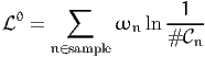 | (3) |
where # n is the number of alternatives available to individual n and ωn is
the associated weight.
n is the number of alternatives available to individual n and ωn is
the associated weight.
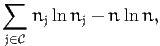 | (4) |
where nj is the number of times alternative j has been chosen, and
n = ∑
j∈ nj is the number of observations in the sample. Note that if some
alternatives are not available for some observations, the formula (4) is not
valid, and the value is not reported.
nj is the number of observations in the sample. Note that if some
alternatives are not available for some observations, the formula (4) is not
valid, and the value is not reported.
 | (5) |
where  0 is the null log likelihood as defined above, and * is the log
likelihood of the sample for the estimated model.
0 is the null log likelihood as defined above, and * is the log
likelihood of the sample for the estimated model.
 | (6) |
 | (7) |
where K is the number of estimated parameters. Note that this statistic is meaningless in the presence of constraints, where the number of degrees of freedom is less than the number of parameters.
The following section reports the estimates of the parameters of the utility function, together with some statistics. For each parameter βk, the following is reported:
The following section reports, for each alternative, its identifier, its name, its availability condition, and the specification of its utility function.
The following section reports, for each pair of parameters k and ℓ,
 | (8) |
 | (9) |
 | (10) |
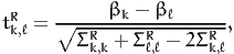 | (11) |
The final line reports the value of the smallest singular value of the second derivatives matrix. A value close to zero is a sign of singularity, that may be due to a lack of variation in the data or an unidentified model.
Under relatively general conditions, the asymptotic variance-covariance matrix of the maximum likelihood estimates of the vector of parameters θ ∈ℝK is given by the Cramer-Rao bound
![{ [ 2 ]} -1
- E [∇2L (θ)]-1 = - E ∂-L-(θ) .
∂θ∂θT](bisonfirstmodel13x.png) | (12) |
The term in square brackets is the matrix of the second derivatives of the log likelihood function with respect to the parameters evaluated at the true parameters. Thus the entry in the kth row and the ℓth column is
 | (13) |
Since we do not know the actual values of the parameters at which to evaluate
the second derivatives, or the distribution of xin and xjn over which to take their
expected value, we estimate the variance-covariance matrix by evaluating
the second derivatives at the estimated parameters  and the sample
distribution of xin and xjn instead of their true distribution. Thus we
use
and the sample
distribution of xin and xjn instead of their true distribution. Thus we
use
![[ ] [ ]
∂2L(θ ) ∑N ∂2 (yin ln Pn (i) + yjnlnPn (j))
E ------- ≈ ----------------------------- ,
∂θk∂θ ℓ n=1 ∂θk∂ θℓ θ=^θ](bisonfirstmodel16x.png) | (14) |
as a consistent estimator of the matrix of second derivatives.
Denote this matrix as Â. Note that, from the second order optimality conditions of the optimization problem, this matrix is negative semi-definite, which is the algebraic equivalent of the local concavity of the log likelihood function. If the maximum is unique, the matrix is negative definite, and the function is locally strictly concave.
An estimate of the Cramer-Rao bound (12) is given by
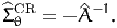 | (15) |
If the matrix  is negative definite then - is invertible and the Cramer-Rao bound is positive definite.
Another consistent estimator of the (negative of the) second derivatives matrix can be obtained by the matrix of the cross-products of first derivatives as follows:
![[ ] n ( ) ( )T
∂2L-(θ) ∑ ∂-ℓn-(θ^) ∂ℓn(^θ-) ^
-E ∂θ∂ θT ≈ ∂θ ∂θ = B,
n=1](bisonfirstmodel18x.png) | (16) |
where
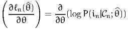 | (17) |
is the gradient vector of the likelihood of observation n. This approximation is employed by the BHHH algorithm, from the work by Berndt et al. (1974). Therefore, an estimate of the variance-covariance matrix is given by
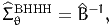 | (18) |
although it is rarely used. Instead,  is used to derive a third consistent
estimator of the variance-covariance matrix of the parameters, defined
as
is used to derive a third consistent
estimator of the variance-covariance matrix of the parameters, defined
as
 | (19) |
It is called the robust estimator, or sometimes the sandwich estimator, due to the form of equation (19). Biogeme reports statistics based on both the Cramer-Rao estimate (15) and the robust estimate (19).
When the true likelihood function is maximized, these estimators are asymptotically equivalent, and the Cramer-Rao bound should be preferred (Kauermann and Carroll, 2001). When other consistent estimators are used, the robust estimator must be used (White, 1982). Consistent non-maximum likelihood estimators, known as pseudo maximum likelihood estimators, are often used when the true likelihood function is unknown or difficult to compute. In such cases, it is often possible to obtain consistent estimators by maximizing an objective function based on a simplified probability distribution.
Berndt, E. K., Hall, B. H., Hall, R. E. and Hausman, J. A. (1974). Estimation and inference in nonlinear structural models, Annals of Economic and Social Measurement 3/4: 653–665.
Kauermann, G. and Carroll, R. (2001). A note on the efficiency of sandwich covariance matrix estimation, Journal of the American Statistical Association 96(456).
White, H. (1982). Maximum likelihood estimation of misspecified models, Econometrica 50: 1–25.


